Ray Tracing

Ray Paths calculated by the Basic Programs †

Results for VLF waves †

Diffusive equiribrium density model †

• Wave frequency : 3.0kHz
• Diffusive equilibrium density model with temperature gradient
• Initial conditions
  • Altitude : 91km
  • Longitude(GM) : 0oE
  • Wave normal direction : (δ,ε)=(0o,0o) : perpendicular to the ground

Results for a dipole field model and the IGRF model from three different initial latitudes are shown in left and right columns, respectively. In each panel, left figure shows a meridian plane in which the ray path is represented by a red line and wave normal directions by blue arrows. Right upper and lower figures in each panel show variations of electron density and reflactive index along the ray path, respectively. Horizontal axes in the right figures indicate propagation times. Regardless of differences of the initial latitudes, all the rays finally arrive at the same L shell.

Initial Latitude(GM)	Dipole magnetic field model	IGRF model
50oN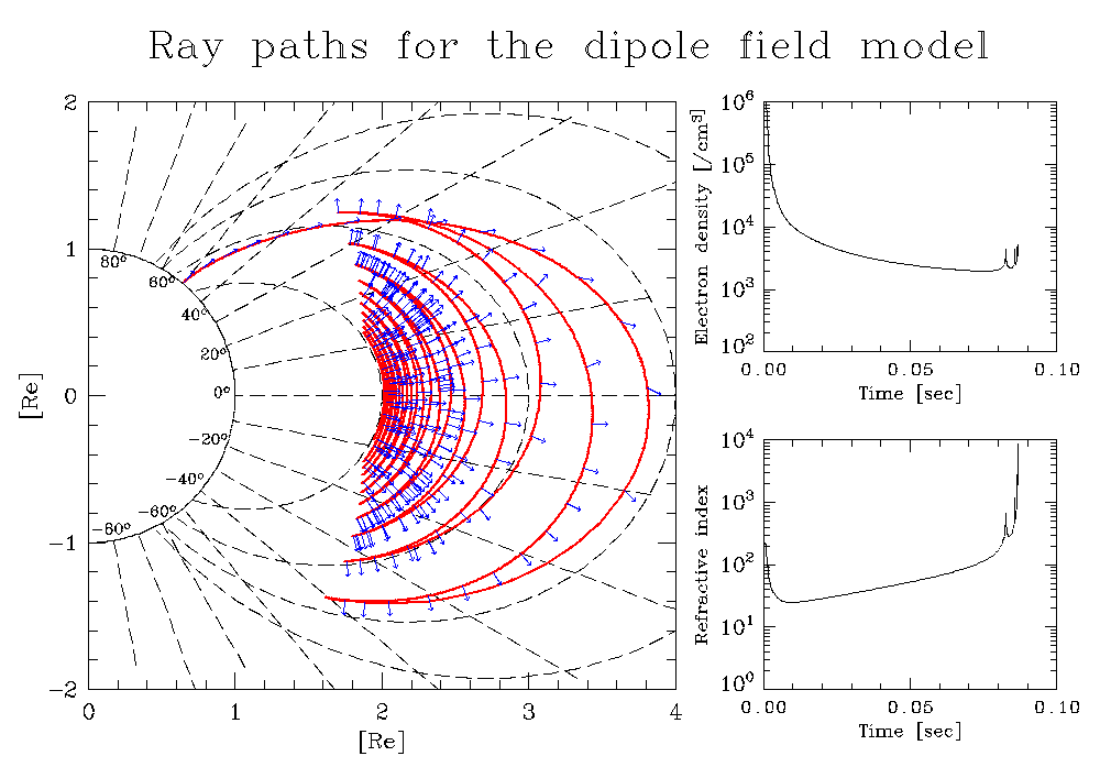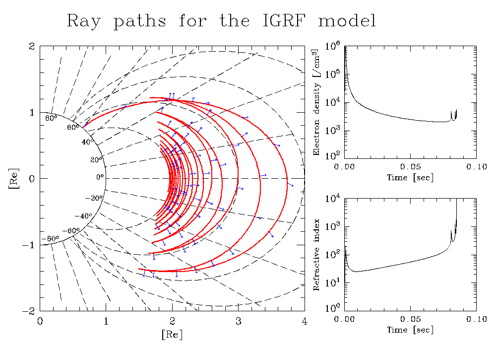
48oN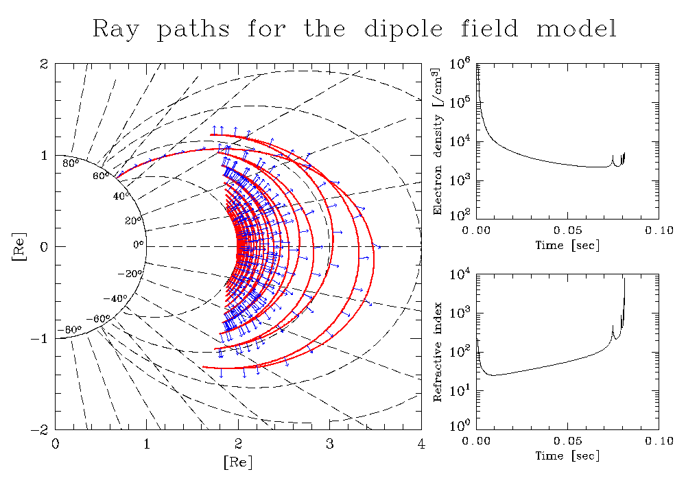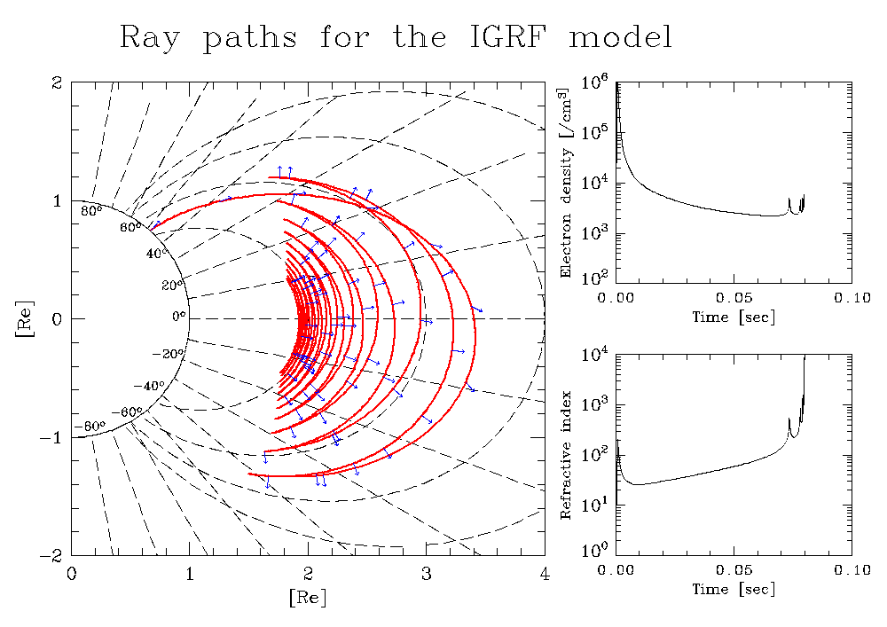
46oN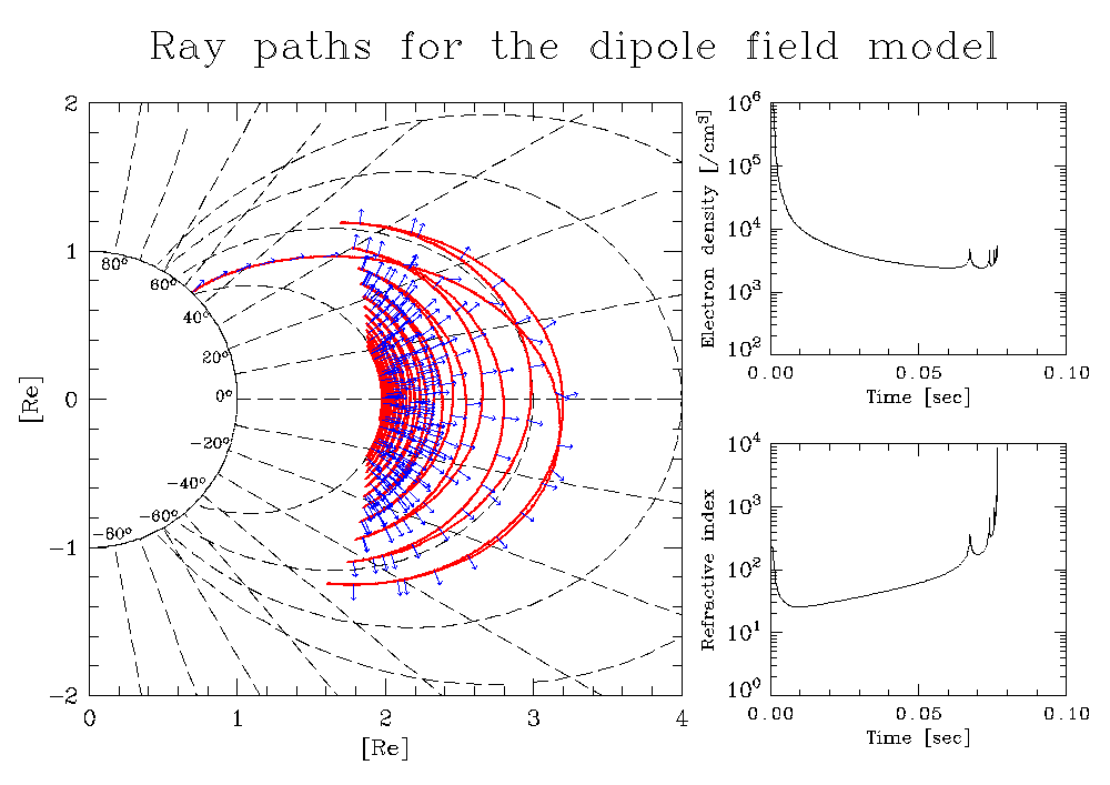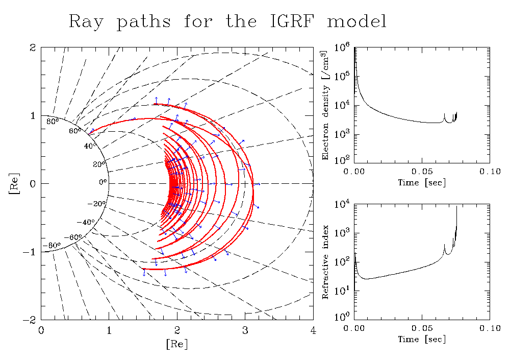

Global core plasma model †

• Wave frequency : 3.0kHz
• Global core plasma model (Date 2000/1/21)
• IGRF model
• Initial conditions
  • Altitude : 91km
  • Latitude(GM) : 50oN
  • Longitude(GM) : 0oE
  • Wave normal direction : (δ,ε)=(0o,0o) : perpendicular to the ground

Results for the global core plasma model in different Kps and local times are shown. Background colors represent electron densities. The ray paths are very complicated compared with the results for a diffusive equiribrium model. In some cases, the rays propagate to the outside of the plasmasphere.

	Kp=0	Kp=3	Kp=6
LT=0hr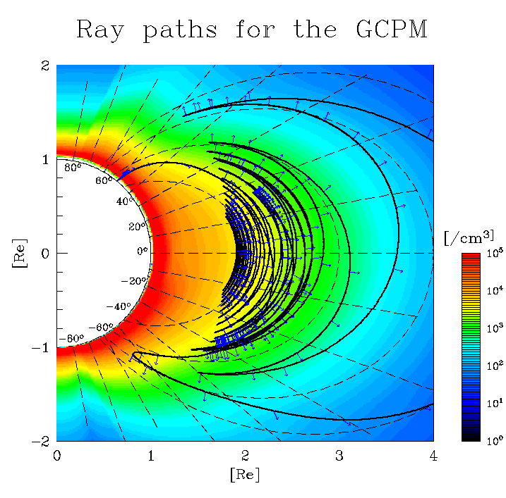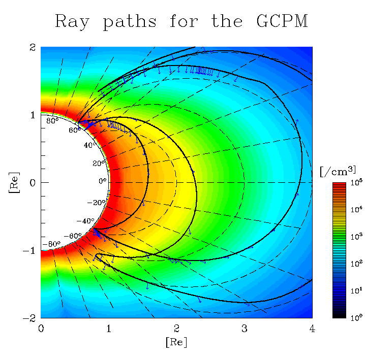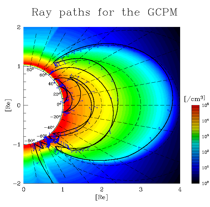
LT=6hr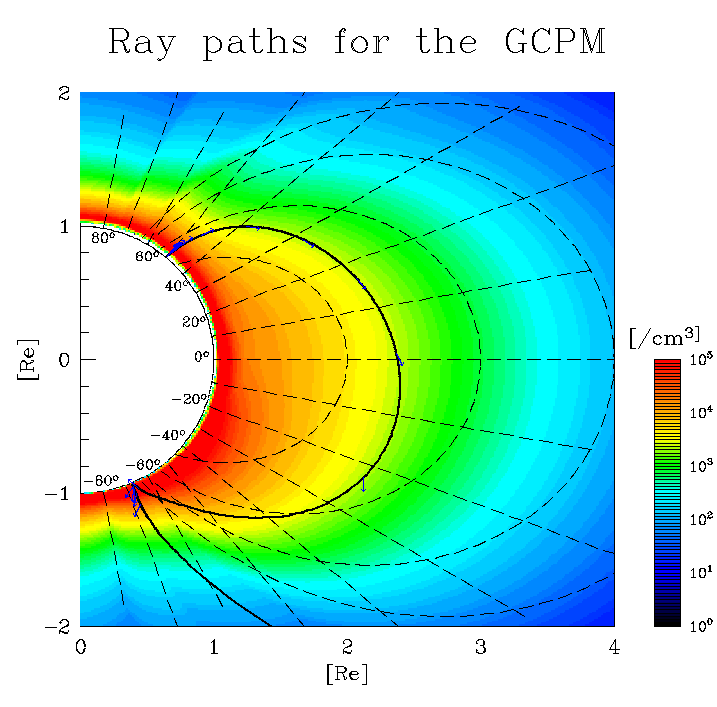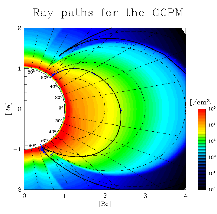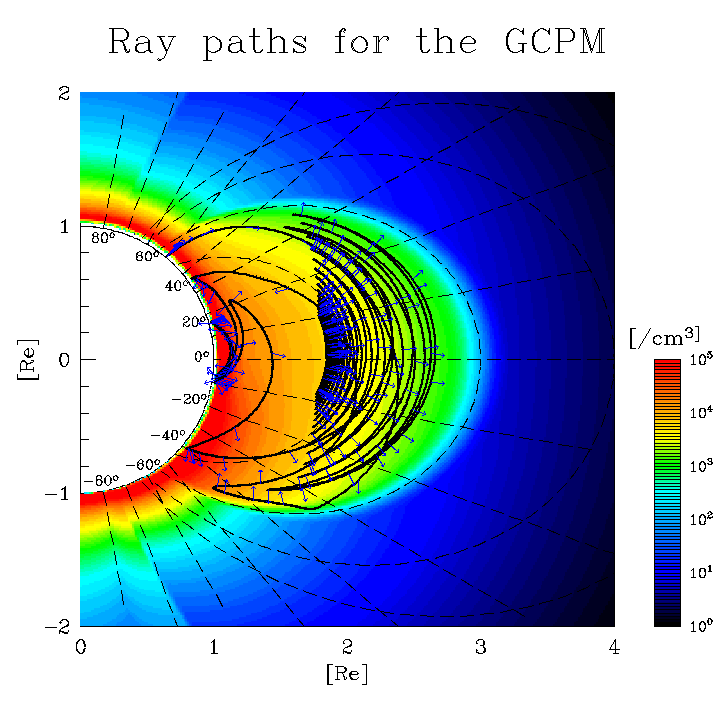
LT=12hr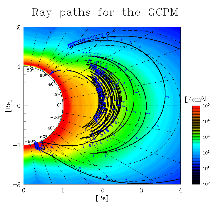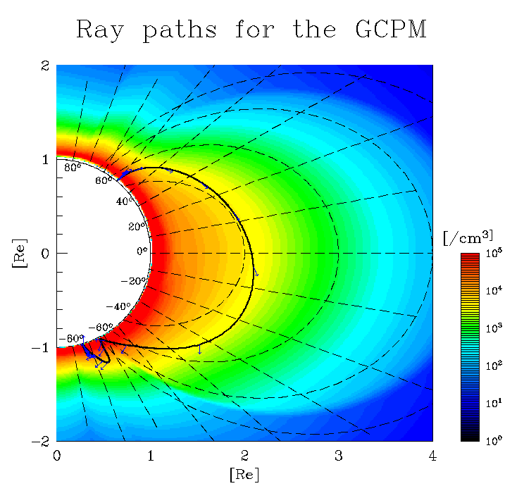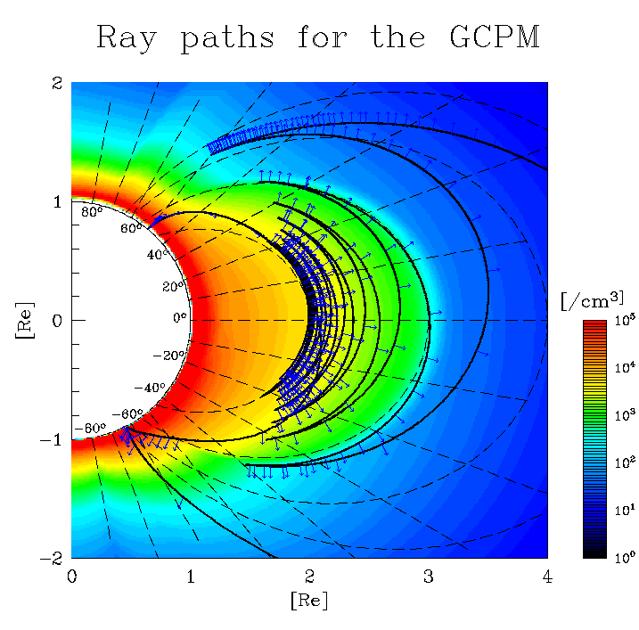
LT=18hr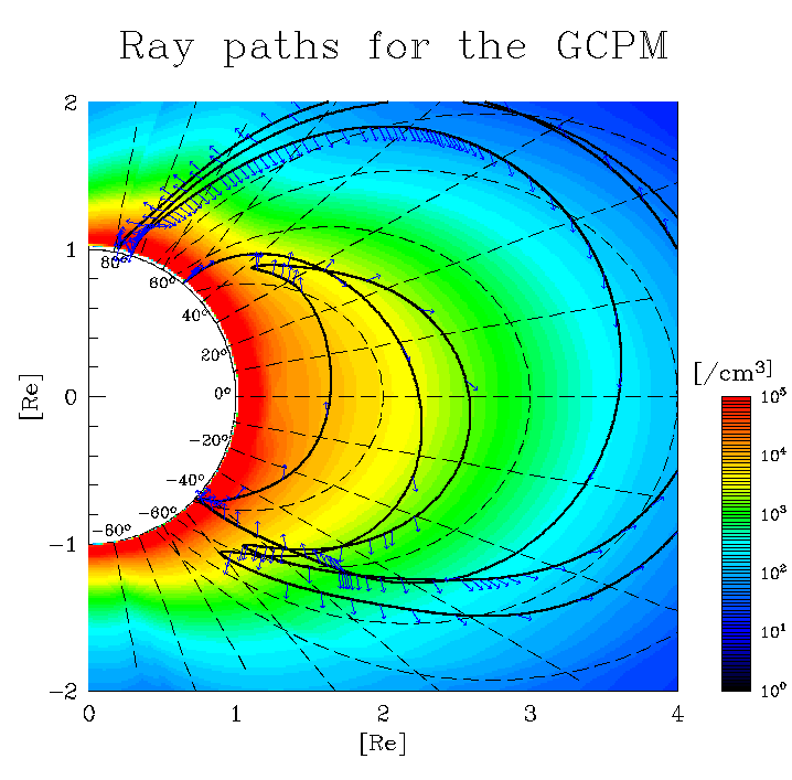

Results for HF waves †

• Wave frequency : 8.0MHz
• IRI density model
• Dipole magnetic field model
• Initial conditions
  • Altitude : 0km
  • Latitude(GM) : 55oN
  • Longitude(GM) : 135oE

Results for ordinary(O-) and extraordinary(X-) modes from different initial wave normal directions are shown in left and right columns, respectively. In the left figure in each panel, a waveguide mode propagation can be seen. The right upper figure in each panel shows electron density at each step of the ray tracing. The right lower figure shows the ray path in a latitude map. In the figure, westward bending is found.

Initial wave normal direction	O-mode	X-mode
(δ,ε)=(50o,0o)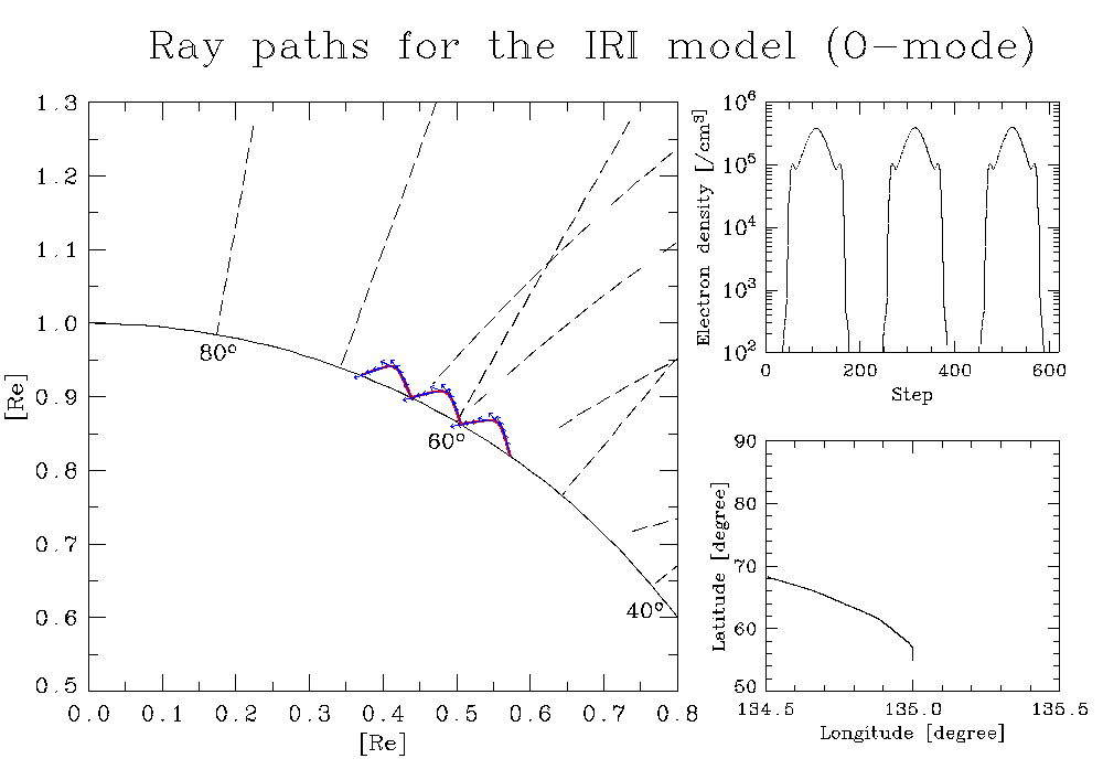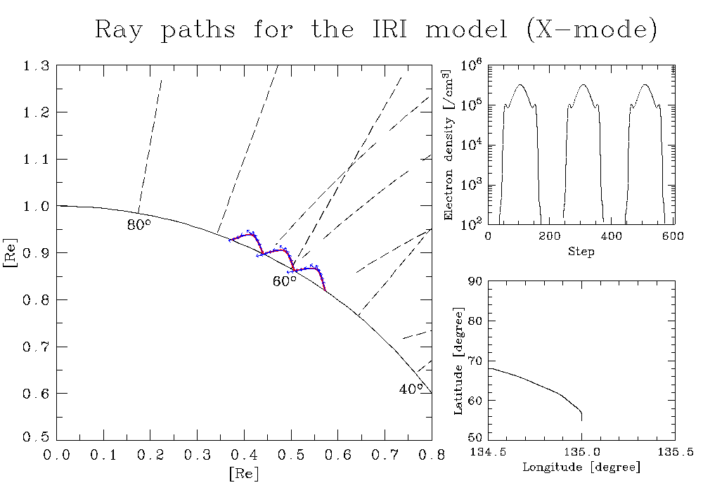
(δ,ε)=(60o,0o)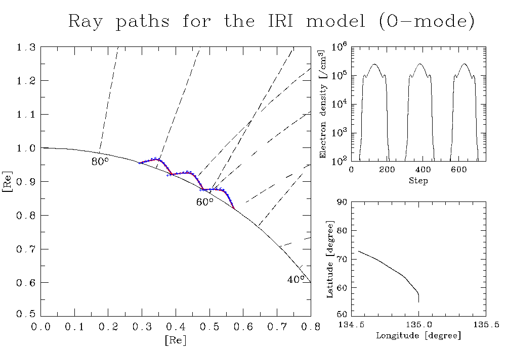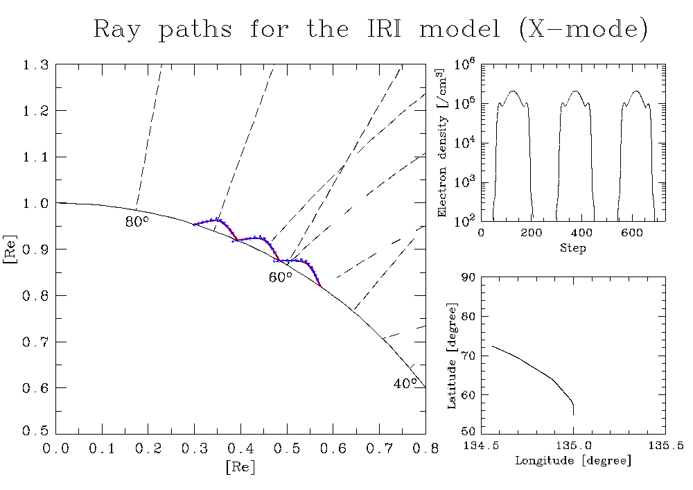
(δ,ε)=(70o,0o)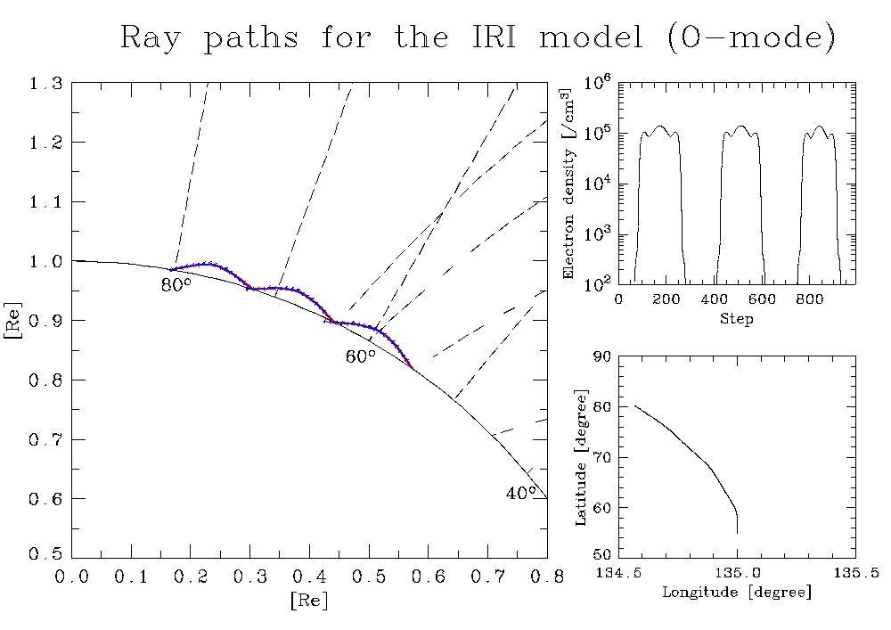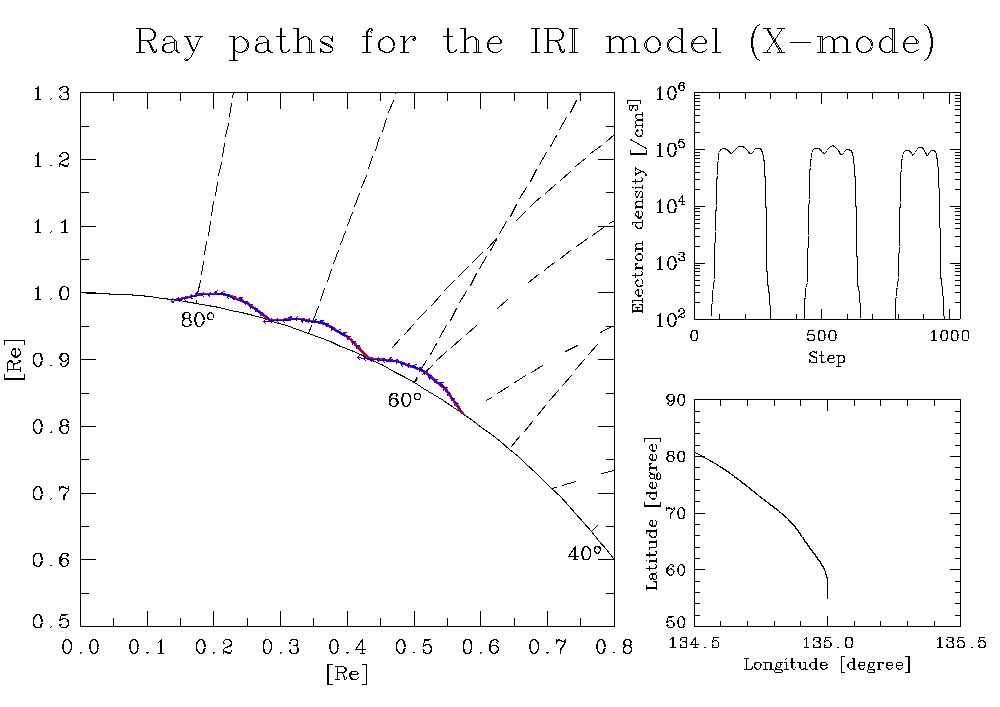

Program to make the figures †

The figures represented above are created by the following C++ program and XYGraph library. The XYGraph is a free graphic library on Linux platforms and the source packeage can be obtained here.

Procedure †

1. Before compiling the program, you have to install the XYGraph package on your computer.
2. Download the source code from here.
3. Compile the source code and make an excutable program

   % cd mkfig
   % g++ mkVLFfig.cpp -lxyg

4. Copy the output file of ray tracing "fort.21" to the directory
5. Run the program
6. Convert the output file format (YACG) into your favorite.