Menu

Technical Description †
1. Introduction †
Fundamental equation of ray tracing originates from the paper by Haselgrove(1954). In the following, however, for the description of ray tracing in the plasma surrounding the earth the contents of the main part of Kimura's paper(1966) will be used. This three dimensional algorithm was first developed for the ray tracing of the whistler mode, but the fundamental equations are applicable to other frequencies, such as HF and higher frequencies. Therefore the following description is mostly common for all frequency ranges in the earth's centered dipole magnetic field model and the diffusive equilibrium plasma model, and one example of ray tracing program is VLF_DE_dipole_F.f shown in the section of Basic Program. VLF ray tracing program is only valid for Extraordinary (X) mode, that is, the right-hand circularly polarized (whistler) mode. DE is the Diffusive Equilibrium model as a plasma density profile, to be described later.
In the earth' environment, the magnetic field lines are deformed from the dipole model and are represented better by so-called IGRF model. For the ray paths of VLF waves in the earth's magnetosphere, the form of the geomagnetic field lines is very much important, so that the dipole model is not enough, e.g. when the actual ray paths of VLF signals transmitted from the ground are compared with those observed by scientific satellites. We have therefore developed another ray tracing program in which the IGRF model is taken into account to get more realistic magnetic field lines. VLF_DE_IGRF_F.f is such a program using DE model as the plasma distribution in a magnetic field model represented by IGRF.
Later, a ray tracing program for HF and higher frequency waves will also be shown for right-handed polarized (R or X-mode) and left-handed polarized (L or O-mode). O- and X- modes are the Ordinary and Extraordinary modes of radio waves in the magnetized plasma.
2. Fundamental Algorithm for Ray Tracing in Plasma Environments Surrounding the Earth †
2.1 Differential Equations for Ray Tracing †
According to Haselgrove (1954) and Yabroff (1961), the series of differential equations determining the ray path in a known plasma distribution around the earth and a known magnetic field model in three dimensional polar coordinate system are represented by the following equations:

The refractive index μ is obtained from the following equation in μ2 [Hines, 1957]:

where
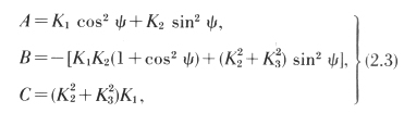

ψ=the angle between the wave normal and the magnetic line of force. Here f0i and fHi are the plasma frequency and cyclotron frequency of the ith constituent (the subscript i refers to electron and ions), and are given by
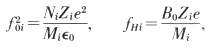
where Ni, Mi are the number density and mass of the ith component, and the particle charge is set equal to Zi times e, where e is the charge of an electron; B0 is the field intensity of the static magnetic field and ε0 is the dielectric constant in vacuum. In (2.4), the effect of collisions is disregarded, but it can be taken into account (see Kimura; 1966).
Since (2.2) generally yields two modes, the ordinary and extraordinary, the propagating mode must be correctly chosen in the ray tracing. For the extraordinary mode, the right handed circulary polarized mode, like whistler mode in VLF frequencies, the following explicit formula for μ2 is adopted.

(These two formulas are equivalent but are written in this fashion for computational accuracy.) The above refractive index formula correspond to the so-called X- mode. In the space above the bottom of the ionosphere, only X-mode is present for VLF waves. However, for HF or higher frequencies, both O-mode and X-mode are present in general. For X-mode, the the above same formula of refractive index can be used, and for O-mode, the sign before the square root term must be reversed.
The derivatives of μ with respect to each component of the refractive index vector ρk appearing in (2.1) are obtained by

where the subscript k corresponds to the coordinates r, θ, φ, and where Y0k is the direction cosine of the magnetic field vector. It should be noted that when ψ→ 0,
 → 0,
→ 0,  → ∞, but
 → 0.
The derivative of μ with respect to ψ is
calculated from (2.2) by the following equation:
→ 0.
The derivative of μ with respect to ψ is
calculated from (2.2) by the following equation:
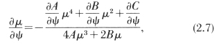
and
 is calculated by

where
 are obtained in the same way as in (2.7).
The derivatives of Xi are determined
by the space variation of electron and ion densities.
are obtained in the same way as in (2.7).
The derivatives of Xi are determined
by the space variation of electron and ion densities.
2.2 Earth-centered Dipole Field Model †
If the magnetic field is assumed to be that of an earth-centered dipole, Yi and Yok in the above (2.4) are given by

The derivative of Yi and ψ are as follows:

2.3 Group Refractive Index and Group Delay Time †
The group refractive index μg is given by

where  is obtained in the same way as , that is,
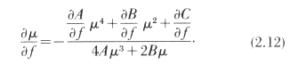
Then the group delay T is computed by
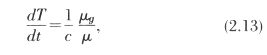
where c is the speed of light.
2.3 Diffusive Equilibrium Model for Plasma Distribution around the Earth †
A diffusive equilibrium (DE) model is a theoretical model in the exosphere, in which the outward motions of plasma constituents, such as protons, helium ions and oxygen ions with their own temperatures are balanced with gravity along a magnetic field line. This model was developed by Angerami and Thomas (1963 & 1964).This model is valid above the top of the ionosphere, say, several hundred km. Therefore in order to extend this model simply to the bottom of the ionosphere, we have to multiply a function decreasing toward zero at the bottom of the ionosphere to the DE model. This function is called as Lower Ionosphere(LI) Model which is explained in section 2.4. In case we have to use a plasma model which is dependent on the latitude, we are able to multiply a latitude dependent function to DE model. In any case, from the algorithm of ray tracing, the derivatives of electron and ion densities with respect to the space coordinates are required. Therefore, if the plasma distribution is represented by any function dependent on the space coordinates, the derivatives can be easily calculated. This model becomes versatile by selecting parameters included in the above functions properly. In case, if we have to use any arbitrary numerical plasma density model, the spatial derivatives have to be numerically calculated. Such a case will also be introduced later in other section.
If the electron density at any altitude is determined by the charge balance with the positive ions, the normalized electron density is determined by

where z is the geopotential height given by

with r0 being a reference radius distance.This expression can be obtained from Angerami and Thomas (1964), eq(B4), by neglecting the centrifugal force which arises from the earth's rotation. In (2.14), i corresponds to each ion, Hi and ηi indicate the scale height and the percentage of the ith ion at the reference level r0. The relative density of the ith ion with respect to electron density is given by
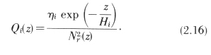
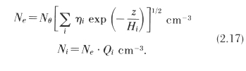
Then the absolute electron and ion densities are
The scale height Hi is a function of the temperature Ti and mass Mi of the ith ion and gravity at r0:
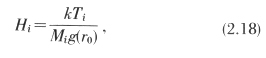
where k is Boltzmann's constant.
2.4 Low Altitude Model for the Electron Density Extended to the Lower Ionosphere. †
In the DE Model so far described, the electron density increases exponentially towards lower altitudes. However, actual electron density in the ionosphere shows a maximum around the so-called F2 layer and decreases toward lower altitude, finally becoming zero at the bottom of the ionosphere (say, around an altitude of 70km). Such an electron density model can be expressed by multiplying the following function Li (Lower Ionosphere(LI) Model as mentioned earlier) to the DE model density represented by (2.19).

In this function Li(r), the electron density is assumed to become zero below an altitude of 90km.
2.5 Numerical Model in Electron Density in the Ionospheric Altitude Range †
There is a case where we need to do ray tracing for e.g.an HF frequency wave in the classical ionospheric altitude range with an electron density distribution dependent upon latitude, longitude and altitude in a complicated manner, which cannot be represented by a combination of simple functions. In such a case, we have to use an arbitrary electron density distribution or numerical electron density model. To realize such a model, we have prepared numerical data allocated to grid points homogeneously distributed in latitude, longitude and altitude direction respectively. We have tried to create such a numerical model by using the electron densities deduced from IRI model. In the process of ray tracing, we need the spatial gradients of electron density. To determine these spatial gradients, we have to calculate them numerically from the data at the nearest grid points, using proportional interpolation.
3. How to Adopt So-called IGRF Model in the Ray Tracing †
In the previous program developed by Kimura(1966) the earth's centered dipole model is used. Later, Kimura et. al.(1985) developed a computer program, in which the so-called IGRF model was taken into account. This new program was used to find the electron density profile by using the Omega signals (delay time and wave normal direction) observed by Japanese satellite Akebono launched in 1989. In the case that the plasma model in the magnetosphere is a theoretical model like diffusive equilibrium model, the plasma density at each point along a ray path is defined along a magnetic field line passing through the point, so that the plasma densities can not be determined simply by the coordinates along the ray path. For any point in the space where the ray path may reach, the information such as the coordinates (geodetic latitude and longitude) of the end points on the earth surface, of the magnetic field lines must be known. In order to satisfy such requirements, we have to do tracing magnetic field lines passing through the grid points in the space, before the ray tracing starts. As the result, additional tedious process must be added toward the normal ray tracing algorithm. The detail of the process is described in the paper by Kimura, et al.(1985). The standard ray tracing program for VLF waves installed in this open source can be used in either the dipole or the IGRF model, by choosing either "dipole" or "IGRF" in the program, In the IGRF model case, you have to run mesh.f, before hand, for the production of mesh data by doing field line tracing.
4. Ray Tracing for HF and Higher Frequencies in the Dipole Model and Arbitrary Electron Density Model †
One HF ray tracing program for O-mode as well as X-mode waves in the ionosphere determined by numerical data as was mentioned in the previous section 2.5 and in the dipole geomagnetic field model is prepared in the Down Load section. Usually, a ray tracing is started from the ground and the wave is reflected at a certain altitude in the ionosphere back to the ground, though the reflection is dependent upon the wave frequency. The wave reflected from the ionosphere comes back to the ground and is reflected back upwards at the surface of the ground. In our ray tracing program, we can continue the ray tracing with multiple ionospheric and ground reflections up to the maximum number of hops assigned in the main program, under the assumption that the ground is a mirror reflector.
The necessity of numerical ionospheric electron density distribution for a ray tracing especially for HF waves arises when we need to know a lateral deviation of ray paths of trans-equatorially propagating HF transmitter signals due to the longitudinal electron density gradient around the sunrise or sunset time. In this open-source, we have selected a numerical model produced from the IRI model, IRI_UT03_5, in which the mesh points distributed in colatitude from 30 to 150 deg (1deg interval), in longitude from 115 to 155 deg (1deg interval), and in altitude from 70 to 500 km (1km interval). By selecting an appropriate longitude of starting point of ray tracing, say, 135 deg, a fairly big eastward electron density gradient is recognized. This density gradient results in westward bending of HF ray paths. Such an effect will be a cause of the off-great circle propagation of HF broadcasting signals via trans-equatorial propagation.
5 Additional Comments on the Ray Tracing Programs so far explained †
For the VLF ray tracing, the starting altitude is set at an altitude little bit higher than the altitude where the wave frequency f is equal to the plasma frequency fp of electrons; actually 91km of altitude is used for the start point, since the lower boundary (fp becomes zero) of the ionosphere is 90km in the model used. A few km upward shift of the starting altitude does not make any significant difference in the ray path.
More rigorous physical explanation of the start point is as follows. If a VLF wave transmitted at an altitude around the ground, the wave is split into two modes when it enters into the ionosphere where fp > 0, one is right-handed polarized (so-called X- or R) mode and the other is left handed polarized (so-called O- or L) mode. When the ray goes up further, the former mode (X- or R mode) becomes linearly polarized where f= fp and then it becomes O-(or L) mode wave and finally the ray is reflected back at an altitude where the following condition is satisfied.

where fH is the cyclotron frequency of electrons. In our ray tracing, the X- (or R) mode is selected in the subroutine "REF", so that this mode (O- or L mode) reflected back at the above condition is rejected in the ray tracing.
On the other hand, relating to the latter mode (O- or L mode), it becomes cutoff when it goes up to an altitude where f = fp, but above there it is actually transformed to X- or R mode (so-called whistler mode) which can continually propagate upwards. The above mentioned mode-change of the latter mode (O- or L mode) to the whistler mode at around the cutoff condition takes place continually if some collisional loss or tunnel effect is taken into account. However, our ray tracing program which does not include either collisional loss or tunnel effect, rejects this mode too, since the latter mode is originally O- or L mode. Therefore by our ray tracing program, any VLF wave starting from the ground is rejected at an altitude nearly the bottom of the ionosphere and so can not penetrate the ionosphere up to higher altitudes.
Regarding to the HF ray tracing program, our selection of modes in the main program can be either X- or O-mode without any discontinuity of mode up to the ionospheric reflection altitudes, even though the ray tracing starts from the ground. In our HF ray tracing program, the starting points are set as their altitudes to be zero.
For HF or higher frequency range, the geomagnetic field model is not so important compared with the VLF frequency range, so that the dipole model is sufficient.
We have to mention a little bit about the computation time in using our ray tracing programs. In either case of HF or VLF, the computation time necessary is an order of several seconds for one initial condition of wave normal direction, when we use a Personal Computer with Intel(R) T2300@1.66GHz on Microsoft Windows XP system.
The program language used in the programs as mentioned above is Fortran, because these programs were made while Fortran was a widely used computer language. However, even now, Fortran programs can work on a PC by using Cygwin free software. Various graphical softwares, such as gnuplot are also available to test our program.
We are glad if these sample application programs can be used as they are or modified to any other application. Algorithm of Adams-Bashforth predictor method and Adams Moulton corrector method for the numerical solution of multi-element differential equations to be used in ray tracing are described in detail in the bottom of this open source. This part as well as the Basic Program was prepared by Yositaka Goto, collaborator in the preparation of this open-source.
If you feel that some of our programs are useful to your application, please let us know, how they are used and your comments.
************************************************************************ †
The last four references listed hereafter are those introducing application of our ray tracing programs, to determine global electron density profile in the plasmasphere by using the data of Omega signals observed by Akebono satellite. But we have not mentioned the details of the program for that analysis.
Reference List †
Kimura, I.(1966), Effects of Ions on Whistler-Mode Ray Tracing, Radio Science, 1, pp.269-283.
Kimura,I., A. Hikuma, Y. Kasahara, A. Sawada, M. Kikuchi and H. Oya (1995), Determination of Electron Density Distributions in the Plasmasphere by using Wave Data Observed by Akebono Satellite, Adv. Space Res.,15(2), pp.(2)103-(2)107.
Kimura, I., A. Hikuma, Y. Kasahara, and H. Oya (1996), Electron Density Distribution in the Plasmasphere in Conjunction with IRI Model, Deduced from Akebono Wave Data, Adv. Space Res.,18(6), pp.(6)279-(6)288.
Kimura, I., K. Tsunehara, A. Hikuma, Y.Z. Su, Y. Kasahara and H. Oya (1997), Global Electron Density Distribution in the Plasmasphere Deduced from Akebono Wave Data and the IRI Model, J. Atmospheric and Solar Terrestrial Physics, 59(13), pp.1569-1586.
Kimura, I.(1997), Ray Tracing Technique Applied to ELF and VLF Wave Propagation in the Magnetosphere, Discovery of the Magnetosphere, History of Geophysics Volume 7, pp.119-128.