Ray Tracing

Ray tracing for whistler-mode propagation has been performed with the effects of ions included. The method is similar to that employed by Yabroff but for the modification in the refractive index due to ions. Outstanding characteristics of the ray paths in such a medium result from the existence of purely transverse propagation at the lower frequencies. The main purpose of this study is to confirm the Smith interpretation of the "subprotonospheric" whistlers. It is found that an enhancement of electron density at the latitude of interest can support the ray path of the fractional hop as Smith suggested, as well as a possibility of successive echoes through a single path. The effect of collisions on propagation is also discussed.

1. Introduction †

Since Maeda and Kimura [1956] first made a ray tracing for whistlers using a graphical method, more exact calculations have been carried out by Yabroff [1961] and Schmerling et al. [1961] using a digital computer. These ray tracings were based on the magneto-ionic theory of propagation as applied to a monotonically decreasing distribution of electrons in the magnetosphere and to the case in which only the effects of electrons are considered. These computations have predicted that the ray paths may be asymmetric with respect to the equatorial plane, a characteristic not favorable to the explanation of the long-continuing echoes of whistlers and VLF emissions. Smith [1960] described a propagation mechanism involving field-alined ducts which seems to explain satisfactorily many of the observed propagation features of whistlers. A ray tracing that included consideration of the effect of protons was done by Hines et al. [1959]. However, this work involved an investigation of transpolar propagation, which differs substantially from the usual conditions of whistler propagation.

Recently, renewed interest has developed in whistler propagation involving substantial departures from the direction of the magnetic field. A new type of whistler called the "subprotonospheric" or "SP" whistler was identified by observations on an Aerobee rocket, on the Alouette satellite, and through ground observations [Carpenter et al., 1964]. The SP whistlers are usually found to exhibit a number of closely spaced components; the dispersion of the first hop or first component is about 4-5 sec1/2 in the case of Aerobee observations near the lower boundary of the ionosphere, and about 3 sec1/2 in the case of the Alouette observations. It was concluded that the ray paths of SP whistlers are restricted to the region below about 1000 km [Carpenter et al., 1964]. The apparent tendency of the whistler energy to echo back and forth between the bottom of the ionosphere and 1000 km clearly could not be explained on the basis of field- alined duct propagation as this explanation is applied to the usual whistlers observed on the ground. An explanation of the mechanism of the upper reflection of SP whistlers was given by Smith [1964], taking into account the effect of ions and a horizontal gradient of the F layer, and by Cartwright (private communication). As was shown by Hines [1957] when the effect of a single ion is included in the magneto-ionic theory, purely transverse propagation is possible for the whistler-mode wave of low frequency. Therefore, whistler energy may reflect at a rather low altitude, say 1000 km, due to refraction through the region of transverse propagation. The initial purpose of the present work on ray tracing was to confirm the hypothesis of Smith for the SP whistlers, and to investigate other phenomena such as the "transverse" whistler [Carpenter and Dunckel, 1965; Kimura et al., 1965]. In the present work, we have adopted the ray-tracing technique of Haselgrove and Haselgrove [1960], and have used the magnetoionic theory with many ions as developied by Hines. First some ray paths were computed for the same conditions assumed by Yabroff [1961] in order to check the program. Then several paths were computed for various electron and ion density models. The resulting calculations confirmed the explanation of the SP whistler phenomenon described by Smith [1964], and in addition showed many interesting features of the ray paths which had not been predicted. In the following we shall describe the generalized magneto-ionic equations that were used and the technique of ray tracing that has been employed. We shall then introduce electron and ion density models to be used for ray tracing, and discuss the results of the ray-path calculations. The SP phenomenon will be discussed and newly discovered features of the ray paths will be presented. Later the effect of collisions will be considered.

2．Differential Equations for Ray Tracing †

According to Yabroff[1961], the series of equations determining the ray path in a three-dimensional polar coordinate system are:

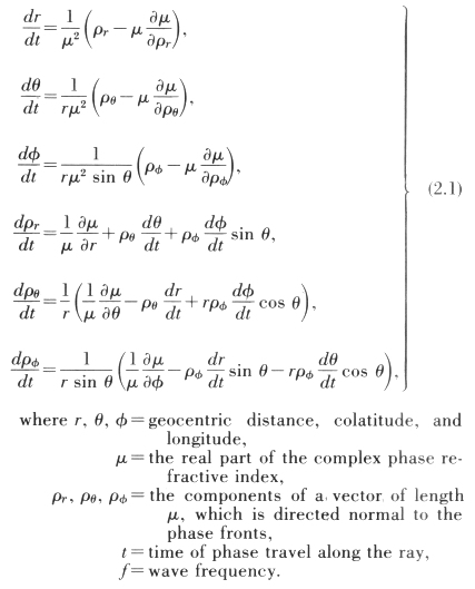
The refractive index μ is obtained from the following quadratic equation in μ2 [Hines, 1957]:

where

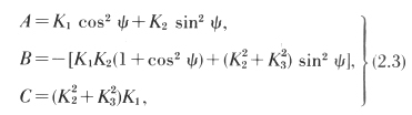
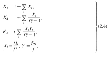
where ψ=the angle between the wave normal and the magnetic line of force. Here f0i and fHi are the plasma frequency and gyrofrequency of the ith constituent (the subscript i refers to each electron and ion), and are given by

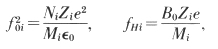
where Ni, Mi are the number density and mass of the ith constituent, and the particle charge is set equal to Zi times e, where e is the charge of an electron; B0 is the field intensity of the static magnetic field and e0 is the dielectric constant in vacuum. In (2.4), the effect of collisions is disregarded, but it will be discussed later. Since (2.2) generally yields two modes, the ordinary and extraordinary, the propagating - or whistler - mode must be correctly chosen in a ray tracing. To do this, the following explicit formula for μ2 is adopted:

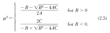
(These two formulas are equivalent but are written in this fashion for computational accuracy.) The derivatives of μ with respect to each component of the refractive index vector ρk appearing in (2.1) are obtained by

where the subscript k corresponds to the coordinates r, θ, φ, and where Y0k is the direction cosine of the magnetic field vector. It should be noted that when The derivation of μ with respect to ψ is calculated from (2.2) by the following equation:

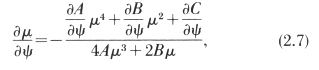
and is calculated by

where are obtained in the same way as in (2.7). The derivatives of Xi are determined by the space variation of electron and ion densities.

If the magnetic field is assumed to be that of an earth-centered dipole, Yi and Yok are given by

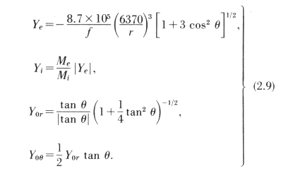
The derivatives of Yi and ψ are as follows:

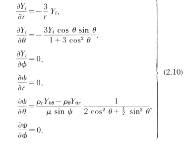
The group refractive index μg is given by

where is obtained in the same way as

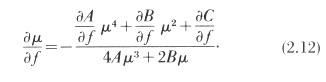
Then the group delay T is computed by

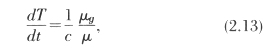
where c is the speed of light.

The frequency limit below which the effect of ions becomes important in ray tracing can be roughly determined by the lower hybrid resonance (LHR) frequency fr [Smith and Brice, 1964], defined by

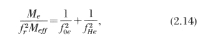
where Me is the mass of the electron and Meff is the weighted mean mass of the ions given by

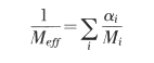
with αi being the fraction of the positive ion density occupied by the ith ion species. At the frequency fr it can be shown that the refractive index in the direction of the static magnetic field is modified, due to ions, only by the amount times that of the case of no ions. Above the frequency fr the modification becomes smaller than this amount. The refractive index in the direction perpendicular to the magnetic field is generally modified much more than in the Longitudinal direction, but it is hard to determine the modific ation analytically. It can be said that above fr there should be no transverse propagation, as in the no-ion case. Therefore, ray paths in the presence of ions for frequencies above fr will not be greatly different from those of the no-ion case. Consequently, a significant effect of ions on the ray paths of the VLF waves may be expected for the frequencies below the lower hybrid resonance frequency. Since the LHR frequency fr depends on foe and Meff, an example of fr as a function of altitude can be illustrated (see fig. 1) by adopting the gyrofrequency at geomagnetic latitude 600 and the electron and ion density profile, which constitutes the I-E model to be explained later. The dashed line of the figure corresponding to the lower part of the I-E model is not always valid because its ion constituent is assumed to be mostly O+. It can, however, be said that in the altitude range indicated, fr should be at least smaller than that shown by the dashed line because the actual effective mass may be larger than that of the oxygen ion.

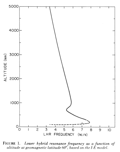
Accordingly, for the above electron and ion density profiles and at dipole latitude 60°, a wave of frequency above 8 kc/s can be considered free from the effect of ions throughout the ionosphere.

If the frequency of interest is always higher than fr over the entire path, the ray path is only slightly affected by the presence of ions. Thus, for many practical purposes, ray paths for frequencies greater than fr may be computed without considering the effects of ions.

3. Method of Digital Computation †

Adam's prediccor-corrector method was used for integration of the differential equations (2.1), and an IBM 7090 computer was utilized.

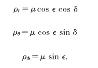
Initial conditions for the start of a computation were determined by assigning the initial wave-normal direction at the starting point (ｒ, θ, φ). This direction is assigned in terms of the angle between the wave normal and the meridian plane, ε deg, and the angle between the projected direction of the wave normal onto the meridian plane and the radial, δ deg. Then the refractive index μ was computed from this wave-normal direction, and the initial values ρr, ρθ, ρψ were obtained from the relations

As Yabroff pointed out, one of the six equations in (2.1) is redundant, so that the magnitude of the wave-normal vector and the refractive index μ are separately obtained. These two values should be identical, but the round-off error which develops during the integrations causes them to differ. In order to keep the two equal, the following correction is made at each step of the integration: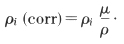

In the earlier computations, ray tracings were started upward from 300 km above the ground, at a level near the maximum of electron density in the F2 layer. Later the ionosphere down to 90 km altitude was taken into account in order to examine the characteristics of the SP whistlers in more detail.

4. Electron and Ion Density Models and Some of the Calculated Ray Paths †

In the program of computation, the electron and ion densities were assumed to have a form,

where Nr and Nθ are functions of the radial distance and the colatitude respectively.

In the case of the ray paths to be shown later, Ne was first assumed constant and several models of the radial variation of electron and ion density were tried.

4.1. Maeda-Yabroff Model (M-Y Model) †

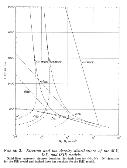
In order to confirm the reliability of our program, the Maeda-Yabroff model of electron density with radius distance r in km was used (see fig. 2), namely,

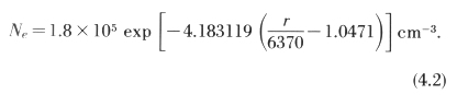
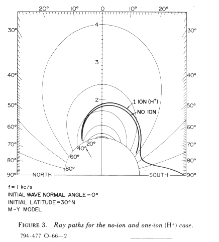
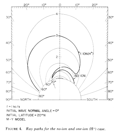
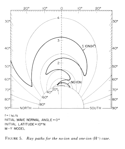
Since our results were found to agree with Yabroffs [1961] to a satisfactory degree, the effect of ions was taken into account by using a model involving protons distributed according to formula (4.2). Figures 3 to 5 show some examples of the ray paths calculated for 1 kc/s under the conditions of protons and electrons only. In these calculations the initial wave-normal direction is vertical (ε=0°, δ=0°) and the starting geomagnetic latitudes are 30°, 20°, and 10°（at 300 km above the ground) respectively. These results show that: (1) the effect of ions on the ray paths becomes more pronounced as the starting latitude decreases; (2) the presence of ions causes the ray to turn at the point where the wave propagates exactly transverse to the magnetic line of force. The ray from latitude 10° shows an oscillatory behavior and does not return to the ground. Such a wave must be absorbed in the magnetosphere because of collision effects. If the frequency of the wave is higher than the lower hybrid resonance frequency throughout the region of the path, the ray surely returns to the ground, just as in the no-ion case.

4.2. Diffusive Equilibrium Model D(I) †

A diffusive equilibrium (DE) model is considered more plausible than the M-Y model above 500 km of altitude [Angerami and Thomas, 1963]. For simplicity in the ealculations, we extended the DE model down to 300 km level. (Actually, along the magnetic line of force this is the more general model, but in this section a spherically symmetric distribution is considered.)

In this model, normalized electron density is determined by

where z is the geopotential height given by

with ro being a reference radius distance. This expression can be obtained from Angerami and Thomas [1964], eq (B.4), by neglecting the centrifugal force which arises from the earth's rotation. In (4.3), i corresponds to each ion, Hi and ηi indicate the scale height and the percentage of the ith ion at the reference level ro. The relative density of the ith ion with respect to electron density is given by

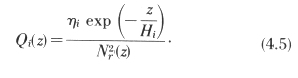
Then the absolute electron and ion densities are

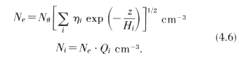
The scale height Hi is a function of the temperature Ti and mass Mi of the ith ion and gravity at r0:

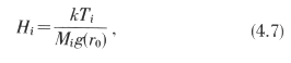
where k is Boltzmann's constant.

The model first chosen is described by

(i) T=1000°K (for all electrons and ions),

(ii) r0=6870 km(h=500 km altitude above the ground),

(iii) Ion composition is O+, He+, H+,

(iv) ηo=1/ηe

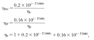
(v) Electron density at η=300 km is taken as 1.8 ×105/cc, which corresponds to Nθ = 3.46×104 in (4.6). The plasma frequency of electrons in this model is also shown in figure 2.

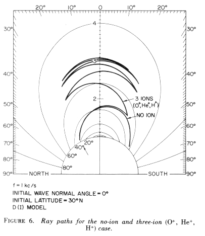
Some ray paths computed on the basis of this model are shown in figure 6. The frequency is 1 kc/s, starting at 30° geomagnetic latitude and the initial wave normal direction is vertical. A pronounced oscillatory feature appears in the ray path. The characteristics of such a path when collisional absorption is considered will be examined in a later section.

4.3. Diffusive Equilibrium Model D(II) †

Another DE model was used for some ray tracing to be explained in section 5. This D(II) model, which is shown in figure 2, is described by

(i) 'T=1000°K,

(ii) r0=7370 km (h=1000 km altitude above the ground),

(iii) Relative ion densities, Qi, at r0, where Qi=ηi, are

(iv) Electron density at h=1000 km is 104/cc, which is Nθ in (4.6).

Though the D(I) model is based on a 500-km reference level, the Qi were computed at the 1000-km level as follows:

4.4. lonosphere-Exosphere Model (I-E Model) †

In addition to the density model above 300 km, a model to cover the lower ionosphere is needed in the ray tracing for the SP whistler study. The following model for the whole altitude range above 90 km was tentatively assumed:

where Nr(D(I)) implies the electron density given by the D(I) model, (4.2), extended down to 90 km (r=6460 km). Here Nr increases with altitude from zero density at 90 km, reaches maximum at about 250 km, and then decreases. This model becomes almost identical with the D(I) model above the altitude of 350 km (see fig. 7).

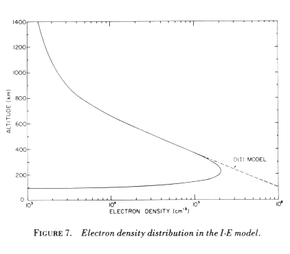
The ion constituents were assumed the same as those above 300 km, and the density percentage was assumed to be given by (4.5), so that below 300 km the major ion was oxygen.

5. Subprotonospheric Whistler †

As was briefly mentioned in the introduction, the SP whistlers are characterized by (1) small dispersion, and (2) multiple echoes. It is also known that the dispersion is increased somewhat at lower frequencies, (see fig. 14) and that the occurrence of SP whistlers is limited to dipole latitudes between about 45° and 650° [Carpenter et al., 1964]. Consequently, it was concluded that this type whistler might be produced only if the ray path were confined to the space below 1000 km altitude and within a small latitudinal range, say 5° or 10°. However, if the ionosphere is considered to consist solely of electrons, it is impossible for the ray to trace such a path. The wave must pass through a region of transverse propagation, where the refractive index would become infinite, in order to be refracted back near 1000 km. Smith[1964] suggested that such a path is possible if the effect of ions is taken into account and also if the wave normal angle with respect to the vertical direction is, say, 15° at a level somewhat above the maximum electron density in the ionosphere. This wave normal angle results from refraction in the F layer when horizontal gradients are taken into account.

An attempt was made to confirm the above hypothesis by ray tracing. In the first calculation, a spherically symmetric model(D(I) model) was assumed, with the ray path starting at 300 km. The effect of horizontal gradients at lower altitudes was simulated by assuming nonvertical wave normal angles at 300 km.

Figure 8 illustrates the ray paths for 0.7, 1.0, and 1.5 kc/s with the initial wave normal angle 20° south (to the right) of the vertical, starting at 300 km above the ground at geomagnetic latitudes of 30°, 45°, 55°, and 65°. These ray paths show that the initial wave normal angle of 20° south of the vertical always causes a southerly bending of the ray and results in the wave returning a little south of the entrance.

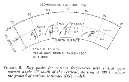
On the other hand, it was found that if the initial wave normal angle was made -20° (north of the vertical), the ray path was bent toward the north and returned to the starting level a little north of the entrance. (The ray path is not shown here.) This fact suggests that the sense of the bending of the ray depends on the sense of the initial wave normal angle from the vertical; in other words it depends upon the sense of the horizontal gradient of the electron density of the ionosphere.

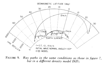
Figure 9 illustrates ray paths calculated by using model D(II). With this model the SP type of ray path appears only at a lower frequency, around 0.7 kc/s, whereas for the D(I) model the SP shape is expected up to at least 1.5 kc/s. An important point here, evident from figure 2, is that in the D(II) model the ratio of electron density at 300 km to that at 1000 km altitude is about 40, whereas in the D(I) model it is 70. It is concluded that the electron density gradient with respect to altitude is also quite an important factor in the production of SP whistlers, and also that a steep gradient favors the production of SP whistlers.

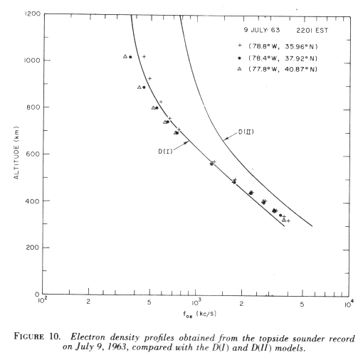
Fortunately, several electron density profiles in the vicinity of Wallops Island, Va. (75°29'W, 37°50'N, geographic) are available from the topside sounder of the Alouette satellite for the time when several SP whistlers were received on an Aerobee rocket. These profiles are shown in figure 10, where the solid lines indicate the D(I) and D(II) model for comparison. It is apparent from the figure that the observed profiles resemble closely the D(I) model, although exhibiting a density gradient somewhat steeper. This implies that the actual density profile is quite favorable to the occurrence of SP whistlers.

The discussion so far has been based on ray tracings started at 300 km altitude with nonzero initial wave normal angle. This approach is still insufficient to completely confirm Smith's hypothesis, because we have not yet checked the effect of the part of the ionosphere below 300 km or the general effect of horizontal gradients of the ionosphere.

To represent the whole of the ionosphere, the electron density (I-E model) expressed by (4.8) is assumed. (Although (4.8) is valid throughout an altitude range above 90 km, the ray tracing using the I-E model was always started from the altitude of 91 km to avoid a computational difficulty at a point between 90 and 91 km where the electron plasma frequency becomes the wave frequency (around 1 kc/s). At that point the refractive index μ would became zero in the absence of collisions.)

Instead of assuming a large initial wave normal angle, a horizontal gradient of the electron density is taken into account [Smith, 1964]. For the sake of simplicity, a horizontal gradient of electron density is assumed to be expressed by the factor Nθ in (4.1), which is only a function of latitude. We first assume that Nθ is a linear function of the latitude θ; that is,

Ne at θ=40°(lat．=50°) becomes twice that at θ=35° (lat.=55°), increasing linearly with decreasing latitude.

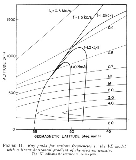
Figure 11 shows the ray paths for the frequencies of 0.7, 1.0, 1.2, and 1.5 kc/s, as well as the contours of constant plasma frequency, where the initial wave normal direction at the entrance was assumed vertical. In this case some higher-frequency paths do not show the SP shape. This fact might indicate that the horizontal gradient around the top of the ionosphere was not sufficient, although the gradient around 1000 km appears to be considerable.

As was mentioned at the beginning of this section, the SP whistlers are usually observed with following echoes, sometimes as many as 10 hops. Such a phenomenon might be due to the lower reflection of the wave upward at a certain point, for example, at the bottom of the ionosphere or by the sporadic E layer. However, as is suggested from the previous ray tracing, a uniform horizontal gradient will result in successive hops in one direction which cannot all be observed at one point, as for instance, by a rocket or a satellite whose horizontal movement is comparatively slow. Consequently, such echoes could be ascribed to a repetition of the wave back and forth along one specific path, such as the usual echoing of the whistler train.

This condition can be realized only by assuming an opposite sense of horizontal gradient at the exit of a path. To test this idea we shall assume a sinusoidal change of electron density with colatitude, for example,

The half period of the sine function was chosen to be approximately equal to the latitudinal interval between the entrance and exit of the one-hop ray path.

Figure 12 shows two ray paths of a 1-kc/s wave starting at the cross points, 55° and 51.3° N geomagnetic latitude, with vertical initial wave normal direction. Contours of constant plasma frequency are also illustrated in the same figure. The two ray paths are almost identical, although the directions of propagation are opposite.

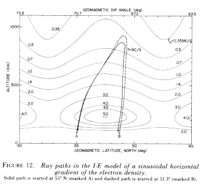
The ray tracing shows that even with a range of wave normal directions at the entrance, the ray paths are nearly identical within 1 percent. This tolerable range of the wave normal angle can be as great as 20° (S) from the vertical, as shown in table 1.

At an exit level, the wave normal angle is as small as 15.6° from the downward direction. Then if there exists a sharp boundary or sporadic E layer, the wave normal might be reflected upward according to the simple Snell's law construction depicted in figure 13．

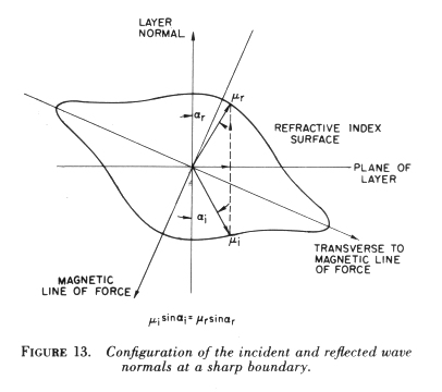
The reflected direction of the wave normal should be a little larger than 15.6° from the upward vertical direction (about 20° (S)). With reference to figure 12, this situation suggests that if a ray starting from A comes down along the solid line path, a wave reflected at B will take the dashed line path, and vice versa.

Consequently, we can conclude that, if the ionosphere exibits the horizontal gradient given by (5.2), then a satellite or a rocket can observe echoing SP whistlers. Naturally, the shape of the irregularity is not limited to the assumed sinusoidal form. The topside sounder record (partly shown in fig. 10) actually indicated a comparable change of the horizontal gradient with latitude, supporting our model.

Table 2 illustrates the computed ray path characteristics, of various frequencies originating at 55.0° latitude, with vertical wave normal direction. In this case, the wave of frequency higher than 3.0 kc/s does not have the SP type of ray path.

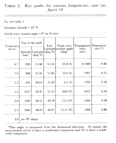
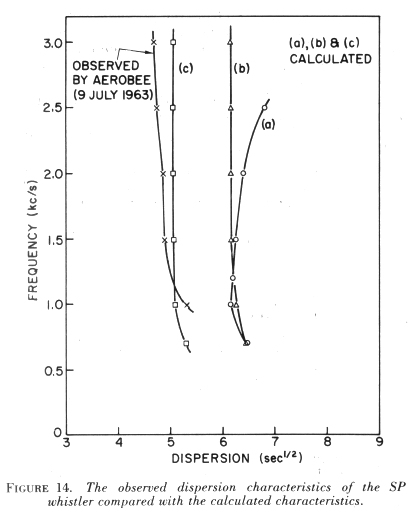
The calculated dispersions in table 2 are plotted as a function of frequency in curve (a) of figure 14. A curve indicated by "observed" shows a characteristic averaged from seven SP whistlers observed by an Aerobee rocket on July 9, 1963. The small difference of the mean dispersion over frequencies between the two curves is due to a difference of absolute electron densities between the actual and the assumed ionosphere. The calculated curve (a) indicates that the dispersion at lower frequencies increases with decreasing frequency, which is similar to the observed curve. However, the calculated dispersion tends to increase at higher frequency, due to the fact that the length of the ray path increases with increasing frequency; moreover, at 3 kc/s no SP shape of ray path can be expected.

If the lengths of the ray paths were the same, the dispersion should be somewhat greater at lower frequencies when the frequency is much less than the lower hybrid frequency, because this is the characteristic of the transverse propagation [Smith, 1964], and the propagation of SP whistlers should become transverse around the top of the ray path. As a result, in order to get the observed characteristics of dispersion, the length of the path should be almost the same over the frequency range of interest.

To realize such a condition let us compute the ray paths for various frequencies which pass the same point at the top, where it is assumed that the wave normal is perpendicular to the magnetic line of force. In this case we can use the same ray tracing program but with a negative increment of the integration. The negative ray tracing shown in table 3 gives the results of such a backward ray tracing from an assumed position of the top of the path. The positive (normal) ray tracing is also used to obtain the other half of the path. In this calculation, the same electron and ion density profiles were used as those for figure 12 and tables 1 and 2．

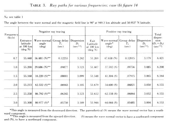
The total dispersion characteristics exhibited by case (b) in figure 14 become preferable to those of case (a) because the dispersion does not increase with increasing frequency at higher frequencies, and the SP type of ray paths can be expected even at 3 kc/s or higher. Curve (c) in this figure is obtained by using one-third times smaller electron density than that used in the previous calculation, in order to reduce the average dispersion of case (b) so as to achieve a better fit to the observed curve.

Moreover, as shown in figure 15, the latitudes of the entrance and exit points in case (b) do not differ much with respect to frequency, in contrast to case (a). Therefore, if we fix the location of the observer at the lower ionosphere, then case (b), or (c), requires only a small range of latitudes at the entrance point, whereas case (a) requires that the latitudes of the entrance point vary widely with frequency, because the ray paths differ so much with respect to frequency.

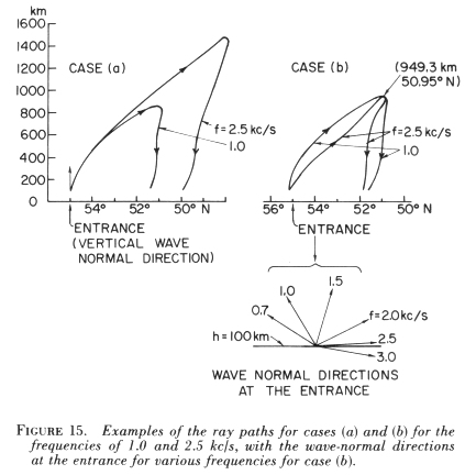
On the other hand, in case (b) or (c) the initial wave normal directions should be different with frequency (see fig. 15), although the wave normal direction in case (a) was assumed the same (vertical) for different frequencies. In case (b) the required wave normal angles change widely with frequency from 56° (N) to 87°(S) for 0.7 to 2.5 kc/s. For 3.0 kc/s, the initial wave normal should be directed a little downward (9°). Such an initial wave normal direction may not be realized by the wave coming from the ground. However, this problem is not serious because, if the location of the apex of the paths is altered toward a little higher altitude, it was shown that the initial wave normal directions would shift counterclockwise, so that we could have any realistic initial wave-normal direction desired.

Now that case (b) or (c), however, is better than (a) from the point of view of the total dispersion characteristics, we must find a mechanism that allows a wide range of the initial wave-normal directions at the entrance in order to support the assumption for case (b) or (c). Two possibilities are suggested. In the first it is assumed that at the entrance there is a "pinhole" window, which may be provided by a small opening in the intense sporadic E layer. If the size of the hole is small compared with the wavelength, the entrance point becomes a point source, so that a wave is able to have any direction of propagation. In the second possibility, the transmitted wave is assumed to be scattered by intense small-scale irregularities in the E region, so that the wave normals are distributed over a wide range of directions. Based on evidence that an intense Es layer was present when some SP whistlers were observed by an Aerobee rocket, one of these mechanisms seems possible.

6. Effect of Collisions †

Throughout the above ray-path calculations the effect of collisions was neglected, since the ray path is actually insensitive to collisions except in the region near the bottom of the ionosphere and at frequencies near the lower hybrid cutoff (resonance frequency).

At 91 km altitude where some ray tracing was started, the electron plasma frequency f0 in the I-E model is 48.3 kc/s and the electron gyrofrequency fH is 1.447 Mc/s. Let us assume that the electron collision frequency ν=4.5×105. Then at f=1 kc/s,

The refractive index μ in this case is approximately given by

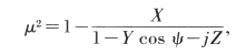
where ψ is the angle between the wave normal and the magnetic line of force. (In this section, “μ” will be used as the complex refractive index. In previous sections, it represented the real part of the index.) In the case where ψ is 60°, we get

Thus the effect of collisions on the real part of μ is less than 1 percent; at a higher altitude, the effect is much less. Consequently the neglect of collisions in the ray tracings appears to be reasonable.

At the lower hybrid-cutoff condition, the effect of collisions becomes predominant, as will be shown later. However, at this condition the ray tracing was stopped so that the ray paths obtained to that point were not seriously affected by collisions. On the other hand, the effect of collisions cannot be ignored insofar as the absorption of the wave through propagation is concerned, since the wave takes a path like those shown in figures 3 to 6．

6.1. Attenuation Due to Collision †

When the collision frequency is taken into account, (2.4) should be changed as

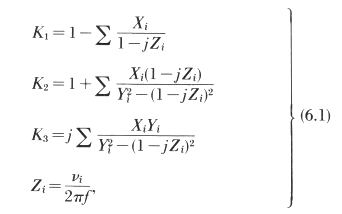
where Xi, Yi are defined in (2.4) and νi is the collision frequency of the ith constituent with the other constituents. For example, in the case of the Coulomb collision which is applicable above the F2 layer, νe is the collision frequency of electrons with other ions and is approximately given by [Nicolet, 1953]

where ne is the electron density and T is the temperature of the plasma.

In the case of the plasma consisting of electrons and protons, the effective collision frequency of protons with electrons should be (see, e.g., Ferraro and Plumpton [1961])

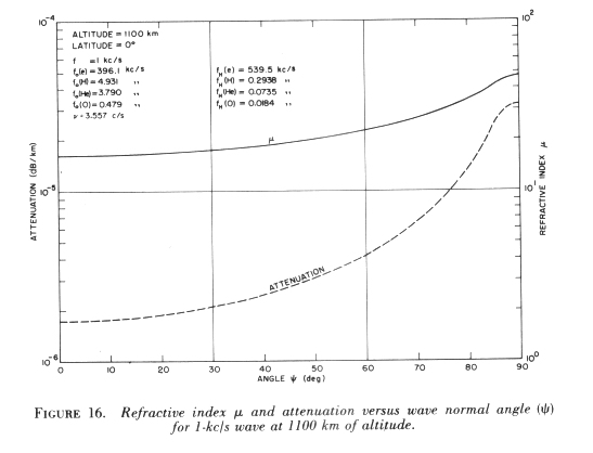
The effect of νp on the attenuation is, then, negligible compared with that of νe. Consequently, an estimation of attenuation was made only taking account of νe given by (6.2). Figures 16 and 17 show the refractive index and attenuation (dB per km) with varying wave normal angles ψ, at the altitudes of 1100 and 13,000 km, where the D(I) model was adopted. From this calculation we found that the real part of the refractive index is almost identical with that obtained for the zero-collision case, except in the vicinity of the lower hybrid cutoff. This result substantiates the rationality of neglecting collision frequency in the ray tracing.

Attenuation (dB per km) for purely transverse propagation was also computed with altitude as shown in figure 18, for the D(I) model.

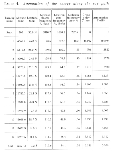
The results given in figures 16-18 indicate that the attenuation becomes appreciable in the case of the lower hybrid-cutoff condition. Therefore an integration of the attenuation Γ in dB over a ray path was tried by integrating the following equation:

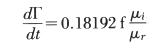
along the path, where μr and μi are a real and imaginary part of μ. Table 4 illustrates the amount of attenuation in every turning point of a ray path shown in figure 6. It is concluded that the amount of attenuation is less than 7 dB until the 13th turning point of the path so that such a "reversing" wave might possibly be observed by using a satellite-borne receiver.

7. Conclusion †

Some interesting features have been revealed as a result of the ray tracing study in which the effect of ions was considered. Ray paths in this case generally differ greatly from those calculated in the no-ion case whenever the frequency is less than the lower hybrid resonance frequency. Some ray paths do not return to the ground but diverge in the exosphere, a feature which seems inconsistent with the fact that whistlers can be observed on the ground. However, it should be noted that most of the whistlers observed on the ground are believed to travel in field-alined ducts which keep the wave normal approximately alined with the earth's field. The characteristics of some whistlers observed by a space vehicle are similar to those predicted for nonducted propagation.

The ray tracing study has supported Smith's hypothesis for SP whistlers, although it was found that a very critical density profile is necessary to get the observed dispersion characteristics with frequency and the echoing features. The topside sounder record of the ionospheric electron density appears to support such a specific model of the ionosphere.

The effect of collisions on the ray path itself was found to be negligible. Collisional effects were found to produce moderate, but not severe, attenuation of the wave.

---

The author expresses his thanks to Professor R. A. Helliwell for his guidance and encouragement of this work, to Dr. R. L. Smith for his helpful advice and criticism throughout the work, to Dr. D. L. Carpenter and Mr. J. Katsufrakis for their aid in supplying experimental data and for their continuing interest, and to Mr. J．Angerami for his helpful advice regarding the appropriate electron and ion density profiles.

Also gratefully acknowledged is the courtesy of the Canadian Defence Research Telecommunications Establishment, Ottawa, Ontario, Canada, in providing the topside sounder data coincident with some SP (subprotonospheric) whistler observations by an Aerobee rocket.

This research was supported in part by the National Aeronautics and Space Administration under grant NsG 174-61 and in part by the National Science Foundation Office of Computer Sciences in the Mathematical Division under grant NSF GP-948.

8. References †

Angerami, J. J., and J. O. Thomas (Dec. 1963), The distribution of ions and electrons in the earth's exosphere. Tech. Rept. No. 3412-3, Radioscience Lab., Stanford Electronics Labs., Stanford University, Stanford, California. Also (Nov. 1964), J. Geophys. Res. 69, No. 21, 4537-4560.

Carpenter, D. L., and N. Dunckel (Aug. 1965), A dispersion anomaly in whistlers received on Alouette 1, J. Geophys. Res. 70, No. 15, 3781-3786.

Carpenter, D. L., N. Dunckel, and J. F. Walkup (Dec. 1964), A new phenomenon: whistlers trapped below the protonosphere, J. Geophys. Res. 69, No.23, 5009-5017.

Cartwright, D. G. (May 1965), Unusually short whistlers observed in the ionosphere, J. Geophys. Res. 70, No. 9, 2249-2250.

Ferraro, V. C., and C. Plumpton (1961), An Introduction to Magneto Fluid Mechanics (Clarendon Press, Oxford, Eng.).

Haselgrove, C. B., and J. Haselgrove (1960), Twisted ray paths in the ionosphere, Proc. Phys. Soc. London 75, 357-363.

Hines, C. O. (1957), Heavy-ion effects in audio-frequency radio propagation, J. Atmospheric Terrest. Phys. 11, No. 2, 36-42.

Hines, C. ０.， W. C. Hoffman, and H. Weil (1959), Transverse whistler propagation, Final Rept. No. 2894-1-F, Res. Inst., Univ. of Michigan, Ann Arbor, Mich.

Kimura, I., R. L. Smith, and N. M. Brice (Dec. 1965), An interpretation of transverse whistlers, J. Geophys. Res. 70, No. 23, 5961-5966.

Maeda, K., and I. Kimura (1956), A theoretical investigation on the propagation path of the whistling atmospherics, Rept. Ionosphere Space Res. Japan 10, 105-123.

Nicolet, M. J. (1953), The collision frequency of electrons in the ionosphere, J. Atmospheric Terrest. Phys. 3, 200-211.

Schmerling, E. R., R. Goerss, S. Miluschewa, P. Riedinger, and I. Pikus (1961), Ray tracing for whistler-mode signal at low frequencies (private communication).

Smith, R. L. (July 1960), The use of nose whistlers in the study of the outer ionosphere, Tech. Rept. No.6, AFOSR-TN-60-861, Radio- science Lab., Stanford Electronics Labs., Stanford University, Stanford, Calif.

Smith, R. L. (Dec. 1964), An explanation of subprotonospheric whistlers, J. Geophys. Res. 69, No. 23, 5019-5021.

Smith, R. L., and N. M. Brice (Dec. 1964), Propagation in multi-component plasmas, J. Geophys. Res. 69, No. 23, 5029-5039.

Yabroff, I. (1961), Computation of whistler ray paths, J. Res. NBS 65D (Radio Prop.), No. 5, 485-505.