Ray Tracing

A three dimensional (3-D) ray tracing technique for whistler mode signals in the earth magnetosphere using a non-dipolar geomagnetic field model is investigated. A difficulty arising from the adoption of a general field model in ray tracing is that field line tracing is additionally required at every step of the calculation. This is because the plasma density profile such as the diffusive equilibrium model are defined along a geomagnetic field line which cannot be analytically determined in the general field model. To substantially reduce the computer time a minimum number of field line tracing are made in advance, and in the course of ray tracing some interpolation is utilized. The error arising from such interpolations is checked and is found to be insignificant. Some examples of ray tracing are shown. The ray path of 5 kHz signals starting from the bottom of the ionosphere of the Siple (64.9°S, 7.5°W in geomagnetic coordinates) meridian is found to deviate eastward by about 15° at the apex.

1. Introduction †

Ray tracing of the whistler mode waves in the magnetosphere surrounding the earth using a computer technique was first made by Yabroff (1961). Later, the effects of ions in the plasma were taken into account by Kimura (1966). These computer programs have been widely used to interpret various whistler mode phenomena.

Analytical models of the geomagnetic field and ion densities in the medium are required in these calculations. Thus far, a dipole model has been assumed for the geomagnetic field and a diffusive equilibrium model for plasma density. Most of the ray tracings have been made in a two dimensional (2-D) frame, such as in a geomagnetic meridian plane.

The actual geomagnetic field is significantly non-dipolar and strongly dependent on the longitude as shown in Fig. 2 (this figure will be explained in detail later). The plasma density depends on local time or longitude leading to sharp density gradients in the longitudinal direction, particularly around the sunrise and sunset hours. Under such circumstances, 3-D ray tracing using a more realistic geomagnetic field and plasma density models is necessary for detailed studies of whislter mode wave phenomena, e.g., tracing the ray paths of a ground based VLF signal observed by scientific satellites.

In this study, the ray tracing program is improved to accommodate a more realistic geomagnetic field model, including higher spherical harmonic components in addition to the dipole term. A more realistic electron density model is also used.

2. Fundamental Equations for 3-D Ray Tracing †

3-D ray tracing equations are represented as follows (Haselgrove, 1955):

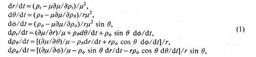
where r, θ and φ are the geocentric distance, geomagnetic colatitude and geomagnetic longitude, μ is the refractive index and ρr, ρθ and ρφ are r, θ and φ components of the refractive index vector ρ(|ρ|=μ). The refractive index μ is determined by the double quadratic equation

in which A, B and C are functions of plasma and cyclotron frequencies of electron and ions, and of the angle ψ between the geomagnetic field direction and the refractive index vector ρ. The angle ψ is given by

where Br, Bθ, Bφ are r, θ, φ components of the geomagnetic field vector BT. In the dipole model, Br and Bθ are represented by a simple function of θ only and BΦ=0.

The electron and ion densities above the top of the ionosphere are often approximated by the following diffusive equilibrium model (Angerami and Thomas, 1964) that represents electron and ion density profiles along the geomagnetic field lines.

where Nde and Ni, are the electron density and the ion density of the i-th species. ηi is the relative density of the i-th ion (i.e., Σ ηi=1). Hi is the scale height of the i-th ion, given by

where k is the Boltzman constant, Ti, and mi, are the temperature and the mass of the i-th ion, and g(r0) is the gravitational acceleration at a radial geocentric distance of reference level r0. For the ion species, only H+ , He+ and O+ are considered. The geopotential height z in Eq. (4) is determined by

N0 in (4) is the electron density at z=0 (or r=r0), which can be a function of θ and φ.

The above density profiles are applicable to altitudes above the peak density altitude (~300 km) in the ionosphere. In order to simulate an electron density profile below the peak density altitude, a function NL which decreases with decreasing altitudes, may be multiplied to Eq.(4). In order to simulate the plasmapause, above which the electron and ion densities decrease sharply, a function is multiplied to Eq.(4), which smoothly connects the diffusive equilibrium model with the outside collisionless model (Aikyo and Ondoh, 1971).

In general, if all terms in the right hand side of Eq.(1) can be calculated using plasma parameters and geomagnetic field parameters as mentioned above, the ray paths can be traced by assigning an initial wave normal direction, and by numerically integrating (1), such as by the Adams' predictor-corrector method.

3. Non-Dipolar Model of the Geomagnetic Field †

In the dipole model, a geomagnetic field line passing through a point (r0, θ0) is represented by the following simple function of (r, θ).

On the other hand, a more general geomagnetic field and field lines can be determined in the geographical coordinate system (r, θ, φ) from the following geomagnetic potential V

where a is the mean earth radius, Pnm(Θ) is the associated Legendre spherical harmonic functions of order m and degree n, gnm and hnm are the Gauss coefficients. A small amount of distortion of the earth from a perfect sphere is neglected. The r, Θ, and Φ components of the field (Br, BΘ, BΦ) are given by B=-∇V, or

The Gauss coefficients are adjusted to fit the observed geomagnetic field. In one such geomagnetic field model, called the IGRF (International Geomagnetic Reference Field) model, the coefficients gnm and hnm are known to order and degree of 10 (see e.g., Peddie, 1982). Therefore, in order to use the above expression of geomagnetic field in the ray tracing Eq.(1), the geographical coordinates must be utilized instead of the geomagnetic coordinates. However, the geomagnetic coordinates which refer to the dipole coordinates, are also used for the interpolation to be explained later and for the display of the calculated ray paths. Therefore, a conversion program between the geographic and the geomagnetic coordinates is used.

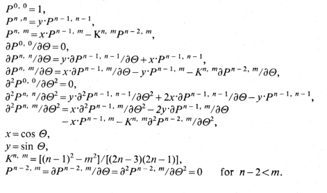
In calculating the right hand side of (1), the derivatives of Br, BΘ, BΦ with respect to r, Θ, Φ are required, so that the 1st and 2nd derivatives of V with respect to r, Θ, Φ must be calculated. The Θ derivatives of Pnm which appear in the 2nd derivatives of V can be calculated by using the following relations (Cain et al, 1967),

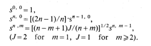
where sn,m is the Schmidt coefficient and Pn,m(Θ) is the Gauss Laplace function, and these quantities are listed in the Appendix (A) and (B), and the derivatives of the Gauss Laplace functions can be calculated by the relations described in the Appendix (B).

4. Problems in Calculating Ray Paths in a Non-Dipolar Model †

All necessary quantities associated with the geomagnetic field can be calculated at any point in the course of ray tracing by specifying the geographical coordinates and assuming an appropriate set of Gauss coefficients, such as IGRF. However, in calculating the plasma density, we need the electron density (N0 in (4)), ion density, and their temperatures at the foot (reference altitude) of the corresponding field line, because the plasma density represented by (4) is the density profile along a geomagnetic field line.

If the plasmapause effect is taken into account, the L value is also needed at each step of the ray path. In the present paper, the L value of a field line is defined as the ratio of the apical distance of each field line to the earth radius.

In the course of ray tracing, the foot point of field line and L value are required for every step of ray tracing. In practice, the following procedure is used in order to reduce the computation time: a minimum number of field line tracings starting from the earth's surface are made in advance before the ray tracing process. On each field line, several mesh points are distributed, at which necessary information of the field line is registered. In the course of ray tracing the information necessary for determining plasma densities is obtained by interpolation from the mesh points. In the following section, the principle of distributing the mesh points and a method for interpolation will be explained.

5. Mesh Points and Interpolation †

The necessary information to be registered at every mesh point is geomagnetic latitude and longitude of the field line at the reference geocentric distance ro, and L value of the field line as previously defined. As a first step, field line tracing is made from the earth's surface every 1° in geomagnetic latitude and every 5° in geomagnetic longitude. We draw latitudinal conic surfaces, with the earth center as the cone top, at every 5° of geomagnetic latitude. All crossing points of the above mentioned field lines and the above latitudinal surfaces become the mesh points. At all mesh points along a same field line, the parameters, i.e., geomagnetic latitude (θ0) and longitude (Φ0) of the field line at the reference radial distance r0, and L value of the field line are common and are, therefore, commonly registered. The geographical coordinates of each mesh point are written in the computer memory.

For interpolation in the course of ray tracing, the geomagnetic coordinates are used. Let Px(rx, θx, Φx) be a point of interest on a ray path. Then two adjacent latitudinal surfaces in geomagnetic colatitudes θ1 and θ2(=θ1+5°) are selected, so as to satisfiy θ1<θx<θ2. On these surfaces, as shown in Fig. 1, Δ points P1(rx, θ1, Φx) and P2(rx, θ2, Φx) are found which have the same rx and Φx. Four nearest mesh points (represented by a rectangle in the figure) are found on each surface. Then on the surface, a radial line passing through the Δ point is drawn, on which line two circle points are determined in the following way of interpolation between the two rectangular symbol points. Namely, the coordinates (r1, φ1) and (r2, φ2) of P11 and P12 points are plotted in an r-φ rectangular coordinate system from which the distance r of the point P1' for φx is interpolated linearly. The coordinates of P1'', P2', P2'' are also determined in the same way.

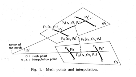
The next step is to interpolate the parameters such as L value and coordinates of the foot point of the field line passing through the point Px from those registered at the eight mesh points (rectangle points) through the circle and triangle points. From P11 and P12 to P1', for example, all parameters are interpolated linearly in φ, and from P1' and P1'' to Pi, they are interpolated linearly in r. From P1 and P2 to Px, the coordinates of the foot point of the field line are interpolated linearly in θ, but L is calculated by a linear interpolation by θ between L1sin2θ1/sin2θx and L2sin2θ2/sin2θx, where L1 and L2 are the L values at the points P1 and P2. In the above processes, L1sin2θ1/sin2θx and L2sin2θ2/sin2θx are the L values at Px estimated from those at P1 and P2, respectively, based on the assumption that the geomagnetic field is approximated by a dipole model. By these procedures, the L value thus interpolated is found to be correct within an error of 0.1%. However, a simple linear interpolation between the L values at P1 and P2 gave rise to an error of about 1% in L value at Px.

The derivatives of electron density with respect to spatial coordinates are also required in the ray tracing process. Some of the derivatives can be obtained analytically but numerical differentiation is also required for some derivatives. For such numerical differentiation, adjacent points around the point Px are selected, for which a similar interpolation is made from the nearest eight mesh points.

6. Validity Check of the Mesh Point Interpolation †

The following ray tracing was made, in order to quantitatively estimate computational error resulting from the interpolation mentioned previously. A magnetic dipole is put at the center of the earth in such a way that the dipole is directed off from the geomagnetic north-south direction by 11° in latitude and 71° in longitude. Such a deviated dipole is intended to simulate an extremely deformed geomagnetic field in the non-dipolar model. The plasmapause location and plasma density distributions are referred to magnetic field lines associated with this dipole.

In such a model, we can trace the ray paths using the conventional 3-D ray tracing program on the dipole model. On the other hand, the same problem is now solved first by distributing mesh points in the geomagnetic coordinate system as explained in the previous section and then by tracing the ray path using our new 3-D ray tracing program, in which the L values and other quantities necessary for determining the plasma densities at each step of the ray path are calculated by interpolation from the mesh point data. Such a comparative ray tracing confirms that the process of interpolation from the mesh points mentioned previously, instead of direct field line tracing at every step of ray tracing, does not cause any serious error in the calculated results.

7. Magnetic Field Lines and Calculated Examples of Ray Paths in the IGRF Model †

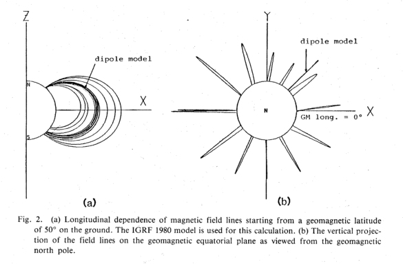
First, Figure 2(a) illustrates a longitudinal dependence of the geomagnetic field lines based on the Gauss coefficients of the IGRF 1980 model (Peddie, 1982) starting at a geomagnetic latitude of 50° on the earth surface. A dipole field line is also shown for comparison. Figure 2(b) is the projection of the field lines on the geomagnetic equatorial plane, as viewed from the geomagnetic north pole. A great difference from the dipole case is evident at certain longitudes. The difference appears to be a minimum at a geomagnetic longitude of ―90°.

Some examples of ray paths calculated in the IGRF 1980 model are shown in Figs. 3 (a) and (b). In this case, an electron density model without latitudinal dependence of N0 in Eq.(4) is adopted for ray tracing, so that the interpolation of parameters using the mesh points was not necessary. Figure 3(a) shows the ray paths of 5 kHz starting from an altitude of 300 km at 50° geomagnetic latitude and at every 30° of geomagnetic longitudes. Figure 3(b) is the projection of the paths on the geomagnetic equatorial plane as viewed from the north pole. In Figs. 3(a) and (b), a ray path in the dipole model is also shown for comparison. The longitudinal dependence of the ray paths shown in Figure 3(a) can be identified by Fig. 3(b).

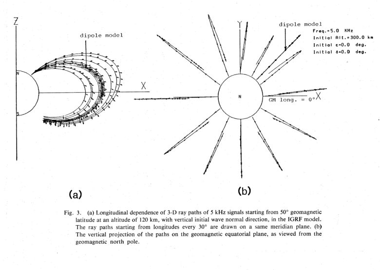
Figure 4(a) illustrates three ray paths of a 5 kHz signal starting from geomagnetic latitudes 55°, 60° and 65° in the meridian of the Siple station (64.78°S, 7.64°W in geomagnetic coordinates) using a plasmaspheric model with the plasmapause at L = 3.2. Figure 4(b) shows the same ray paths projected on the geomagnetic equatorial plane seen from the north pole. As is evident from this figure, the ray paths deviate eastwards by about 15° at the apex of the ray paths. The paths starting from the initial latitudes of 60° and 65° return back to the ground almost at their initial longitude, but the path starting from the 55° latitude further deviates eastwards on its returning path. This substantial eastward deviation is caused by a reflection of the wave normal at the plasmapause. In Fig. 4(a) the location of the plasmapause is represented by thick dashed line. The ray paths starting from the latitudes of 60° and 65° lie completely outside the plasmasphere, so that such an effect is not recognized.

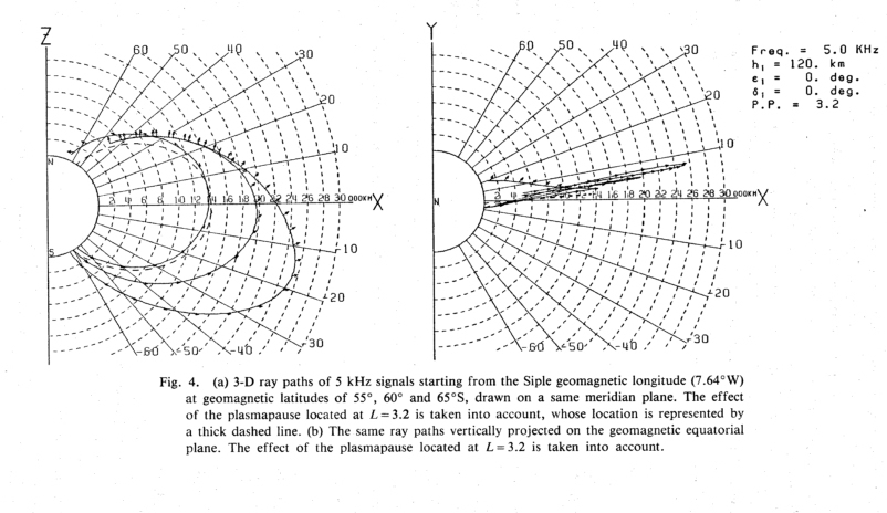
The eastward deviation of the paths starting from the Siple longitude, recognized by ray tracing is consistent with the results of observations by our low inclination and high eccentric satellite EXOS-B (Kimura et ah, 1983), by which the Siple signal was more frequently detected with stronger intensity on the east side from Siple station by 10―15° than on the west side, close to the Siple L value of 4.

8. Discussion and Conclusions †

A 3-D ray tracing program for whistler mode waves in the earth's magnetosphere is modified so as to be applicable to a non-dipolar geomagnetic field model. A plasma density profile to be used for ray tracing is defined along geomagnetic field lines and plasma densities at the base (reference) altitude can be expressed as functions of the coordinates of the foot of each field line.

All parameters such as plasma parameters and their spatial gradients necessary for every step of ray tracing are referred to the geomagnetic field line passing the point on the ray path. Instead of tracing the geomagnetic field line at every step of ray tracing, all necessary parameters referred to the field line are registered at the mesh points that are distributed over the magnetospheric space in advance of ray tracing. Actually the mesh points were distributed every 5° in geomagnetic longitude and in latitude on the field lines starting the earth's surface every 1° in geomagnetic latitude. Such a coarse distribution of mesh points suffices for our ray tracing.

As to the definition of L value, it was found that the L value defined from the geomagnetic equatorial distance of each field line results in much larger computational error in ray tracing, as compared with those L values defined from the apical distance of each field line.

As an application of this technique, ray paths of the VLF Siple signal were calculated and it was found that the paths starting around the longitude of Siple station, Antarctica deviate eastward.

In this study, we have used the Gauss coefficients of the IGRF 1980, which include terms of order and degree of 10. However, in the actual ray tracing it is not necessary to take all such higher terms into account. For example, we could have almost the same results as far as the shape of magnetic field lines is concerned, by taking the maximum degree and order of coefficients to be used for field line tracing as 3 beyond 5 earth radii, as 4 beyond 2.5 earth radii, and as 5 beyond 1.7 earth radii. Therefore, the truncation of the Gauss coefficients in the actual ray tracing can further save computer time. In order to simulate more realistic geomagnetic field in the magnetosphere,

external current source terms, such as due to the ring current and the effect of the solar wind, have to be added to the expression (8). However, these contribution are highly time dependent or dependent on the solar activity. This is an area for future work. Moreover, the main distortion of field lines causing a great change in some ray paths as compared with those in the dipole model, is attributed to the higher order terms which are only effective in the lower part of the magnetosphere, where the effects of the external current sources are relatively ineffective. Therefore, the results of the present study will be relevant at least in magnetically quiet periods.

---

We are grateful to Dr. K. Hashimoto for his valuable comments and discussion. We also acknowledge Mr. K. Yamaashi for his assistance in calculation of a part of ray tracing, Dr. J. P. Matthews for his kind reading of this manuscript, and Mr. Y. Omura for his assistance in editing this manuscript. This work was supported by Grants-in-aid for Science Research project by the Ministry of Education, Science and Culture.

APPENDIX †

(A) Schmidt Coefficients

(B) Gauss Laplace Functions and Their Derivatives

REFERENCES †

AlKYO, K, and T. Ondoh, Propagation of nonducted VLF waves in the vicinity of the plasmapause, J. Radio Res. Labs., 18, 153-182, 1971.

Angerami, J. J. and J. O. Thomas, The distribution of ions and electrons in the earth's exosphere, J. Geophys. Res., 69, 4537-4560, 1964.

Cain, J. C, S. J. HENDRICKS, R. A. Langel, and W. V. HUDSON, Proposed model for the International Geomagnetic Reference Field―1965, J. Geomag. Geoelectr., 19, 335-355, 1967.

Haselgrove, J., Ray theory and a new method for ray tracing, in The Physics of the Ionosphere―Rept. of 1954 Cambridge Conference, pp. 355-364, 1955.

Kimura, I., Effects of ions on whistler mode ray tracing, Radio Sci., 1 (New Series), 260-283, 1966.

Kimura, I., H. Matsumoto, T. Mukai, K. Hashimoto, T. F. Bell, U. S. Inan, R. A. Helliwell, and J. P. Katsufrakis, EXOS-B/Siple station VLF wave-particle interaction experiments: 1. General description and wave-particle correlations, J. Geophys. Res., 88(A1), 282-294, 1983.

Peddie, N. W., International Geomagnetic Reference Field: the third generation, J. Geomag. Geoelectr., 34, 309-326, 1982.

Yabroff, I., Computation of whistler ray paths, J. Res. NBS 65D (Radio Prop.), 485-535, 1961.