Ray Tracing

Adams Method †

1. Fundamental theorem of calculus †

The ray tracing program recursively solves the differential equations in Eq.(2.1) in "Technical Description" by the Adams method which consists of the Adams-Bashforth predictor method and the Adams-Moulton corrector method. Both methods are derived from the fundamental theorem of calculus,

where and .

2. Adams-Bashforth predictor method †

The predictor method uses the Lagrange polynomial approximation for f(t) in Eq.(1-1) based on prior k points ,

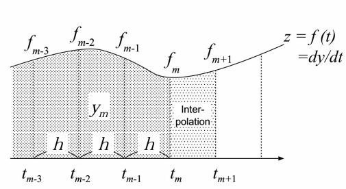
where h shows a step size. A schematic chart of this method is shown in Fig.1. In this process, an extrapolation is used to predict points over the interval [tm, tm+1]. The Adams-Bashforth predictor pm+1 is represented by integrating Eq.(2-1) over this interval:

where

and

In case the step size h is variable at each step, Eq.(2-2) are modified using a divided difference Φi(m) as follow,

where

and

In these equations, the following parameters

and

are used.

3. Adams-Moulton corrector method †

The corrector method also uses the Lagrange polynomial approximation for f(t) in Eq.(1-1). In this case, f(t) is derived from the above-predicted point (tm+1, fm+1) in addition to the prior k points (tm-k+1, fm-k+1),…, (tm, fm). As shown in Fig.2, an interpolation is used to correct the points over the interval [tm, tm+1]. The Adams-Moulton corrector cm+1 is represented by

where

and

In case the step size h is variable, the correlator is represented by using the predictor pm+1 as follows,

where Φk+1p is derived from the same equations as Eq.(2-9) except for defining f[xm+1] as

4. Acceptance of the corrector †

The validity of the k-order corrector is verified by the difference from the (k+1)-order corrector at the same step:

When the ERR is less than a given error ε, the k-order corrector is accepted. On the other hand, when the ERR is greater than ε, estimation of the corrector at the present step is retried with a new order and a step size for the Lagrange polynomial approximation.

5. Determination of the New Order †

Whether the estimated corrector is accepted or not, the order is chosen from among k-1, k or k+1 according to the following conditions. In initial phase, however, the order is increased by 1 regardless of these conditions until the corrector is first unaccepted or k gets 12.

(a) The order k-1 is chosen when one of the following condition is satisfied.

Here, ERK, ERKM1, ERKM2, ERKP1 are defined as estimated errors of k, k-1, k-2 and k+1 order functions for f(t) at tm+1 as

where

(b) The order k+1 is chosen when one of the following condition is satisfied.

(c) The order k is chosen when the conditions (a) and (b) are not chosen

6. Adjustment of the Step Size †

After the estimated corrector is accepted and the next order is chosen, a new step size is determined according to following procedures.

In case the estimated corrector is not accepted, the step size is always set to be a half.

Reference †

Scientific Subroutine Library II (SSL-II) Users Manual, Fujitsu, 1987.